Check your reasoning: Why can one ECG pattern support several diagnoses?

The surface ECG records projected voltage over time. Different anatomy, activation sequences and recording conditions can produce similar shapes; pattern recognition needs clinical context and targeted confirmation.

P → QRS → ST → T

PQRSSTTPRQT
PR: P onset to QRS onset. QT: QRS onset to T end. Original uncalibrated schematic, not a patient tracing; CC BY 4.0 or MIT.

Timing

P waves and their relation to QRS complexes describe atrial activity and conduction. QRS duration describes ventricular activation time. QT contains depolarization and repolarization.

Direction

The same source is viewed through different lead axes. Opposite deflections need not mean different beats. The limb leads describe the frontal plane; chest leads sample different spatial fields.

Amplitude

Voltage depends on the source, geometry, body tissues, electrodes and gain. High voltage is not a direct measurement of wall thickness; low voltage does not identify an infiltrative protein.

Recovery

ST–T shape must be interpreted relative to QRS direction, symptoms and prior recordings. Secondary repolarization changes can mimic primary ischemia.

Check your reasoning: What is the first correction to “the QT measures repolarization”?

QT includes QRS depolarization time. A wide QRS may prolong QT even without the same increase in repolarization time; report QRS duration and choose an appropriate interpretation method.

Chest landmarks

Anterior schematic: patient right is viewer left; V4, V5 and V6 share a horizontal levelRightLeftV1V2V3V4V5V6
Original anatomical schematic. V4–V6 share one horizontal level.

Place V4 before V3

  • V1 / V2: fourth space, right / left sternal border.
  • V4: fifth space, left midclavicular line.
  • V3: halfway from V2 to V4.
  • V5 / V6: level with V4, anterior axillary / midaxillary line.
  1. Prepare the signal. Confirm identity, indication, patient position, skin contact and electrode labels. Support relaxed limbs; reduce movement. Inspect calibration and filters before accepting machine intervals.
  2. Count spaces from a palpable landmark. Find the sternal angle and second rib, then count to the fourth intercostal space for V1/V2. Locate V4 before interpolating V3. Keep V5/V6 level with V4; do not follow a rib downward.
  3. Use standard limb sites. Arms and legs distal to shoulders and hips; wrists/ankles are not mandatory. Torso relocation changes the tracing and must be documented.
  4. Preserve comparability. Record nonstandard sites, gain, speed and patient position. Compare like acquisitions before interpreting a new axis or voltage change.

At 25 mm/s, one small square is 40 ms; at 10 mm/mV, one small square is 0.1 mV. A displayed image may be resized: measure from its printed grid and calibration pulse, not a ruler held against a screen. Place chest electrodes against the chest wall at the anatomical landmarks; breast tissue is not a replacement landmark.

Worked case. A repeat tracing develops an rSr′ in V1 after the electrodes were placed near the clavicles. Inspect and repeat at the fourth spaces before labeling a new conduction abnormality.
Do not overcall. A sudden loss of R-wave progression after reattachment is an acquisition question as well as a clinical finding.
Check your reasoning: Where should V5 and V6 lie relative to V4?

In the same horizontal plane as V4, at the anterior axillary and midaxillary positions; not progressively lower intercostal spaces.

RA ↔ LA cable reversal

  • Lead I flips.
  • II and III exchange.
  • aVR and aVL exchange.
  • aVF stays unchanged.

Chest-lead reference is unchanged; usual R-wave progression can persist.

Mirror-image dextrocardia

Negative I and positive aVR can overlap with arm reversal.

Conventional left-chest R progression is commonly poor or reversed.

Check examination/imaging and label an adapted repeat ECG.

An unexpectedly negative P–QRS–T complex in I and positive aVR should trigger a cable check, especially when the prior ECG had a different orientation. An axis label from the computer cannot distinguish a biological change from a change in the measurement system.

  1. Start with the P wave. Is the apparent atrial axis plausible for the rhythm? Look for coordinated polarity changes rather than an isolated negative QRS.
  2. Inspect all six limb leads. With isolated RA/LA exchange, I is inverted, II/III and aVR/aVL exchange, and aVF is unchanged. These follow directly from the lead equations.
  3. Inspect V1–V6. Isolated arm exchange leaves their reference unchanged. Mirror-image dextrocardia commonly gives poor or reversed progression in conventional left-sided chest leads; other causes of poor progression remain possible.
  4. Trace cables to skin and repeat. Verify chest landmarks too. If dextrocardia is suspected, correlate examination/imaging and obtain an explicitly labeled adapted recording.
Worked case. Lead I becomes entirely negative, but the chest leads match yesterday. A cable check finds RA/LA exchange. The corrected repeat recovers the prior pattern; retain the corrected ECG for serial comparison.
Do not overcall. Chest–limb or ground-electrode exchanges can change reference potentials and distort many leads. Do not salvage precise voltages or QT measurements by simply relabeling an uncertain recording.
Check your reasoning: Does negative lead I alone diagnose dextrocardia?

No. Check the P wave, all limb leads, chest progression, actual cable placement and the clinical anatomy.

High-pass cutoff ↑

Removes slow baseline components.

Tradeoff: phase distortion can alter the ST level.

Low-pass cutoff ↓

Removes rapid signal components.

Tradeoff: QRS notches and pacing spikes can fade.

Baseline wander, muscle activity, loose electrodes and electrical interference can imitate rhythm or repolarization abnormalities. Look across simultaneous leads for native QRS complexes continuing through noise, and relate the pattern to movement and the observed patient. Do not use apparent clinical stability alone to dismiss a dangerous rhythm.

  1. Fix acquisition first. Restore contact, relax/support limbs and inspect cables. Repeat while minimizing motion; preserve the original for comparison.
  2. Read the bandwidth. The high-pass filter sets the low-frequency boundary; the low-pass filter sets the high-frequency boundary. The 50/60-Hz notch targets mains interference.
  3. Choose the diagnostic question. Rhythm monitoring and diagnostic ST/QRS analysis require different fidelity. Retain a standard diagnostic recording when a stronger filter is used to make rhythm visible.
  4. Document the change. Compare recordings with settings shown; an apparent improvement may be a processing effect.

A primary 45-patient experiment demonstrated artifactual ST shifts with a 0.5-Hz high-pass filter in real-time mode. This is a phase-response issue: modern validated digital filtering cannot be judged by the cutoff number alone. A 40-Hz low-pass filter can improve noise but attenuate rapid QRS detail and pacing spikes.

Worked case. ST depression appears only in the monitor’s heavily filtered printout. Repeat a diagnostic 12-lead and compare settings before attributing the difference to dynamic ischemia; symptoms still determine urgency.
Do not overcall. Neither “filtered” nor “unfiltered” guarantees truth. Assess signal integrity and the acquisition method.
Check your reasoning: Which filter is most directly responsible for losing fine QRS notches?

An excessively low low-pass cutoff removes high-frequency detail. High-pass phase distortion is a different mechanism that may alter ST level.

Atrial clock: organized

Repeated atrial events are equally spaced in this conceptual timing strip.

Ventricular clock: irregular

Unequal RR intervals do not establish AF. Compare the atrial activity and conduction.

Original teaching schematics, not patient recordings. CC BY 4.0 or MIT. Timing and voltage are illustrative unless explicitly labeled.

  1. Is the ventricular rhythm regular?

    Use a long strip and actual RR measurements. Look beyond one short sample.

  2. Is atrial activity organized?

    Inspect several leads for consistent P waves, flutter activity, premature atrial beats or a rhythm marching through artifact.

  3. How do atria and ventricles relate?

    A fixed relationship, variable conduction, nonconducted premature P wave or independent rhythms can explain the same pause.

AF pattern

Disorganized atrial activity, no consistent P-wave pattern and irregular ventricular intervals when AV conduction is present. Confirm visually; a machine label is insufficient.

Exceptions that matter

AF can have a regular ventricular rhythm with complete AV block or pacing. Flutter with variable AV conduction can look irregular. Artifact can mimic fibrillation.

A strip is irregular, but identical atrial waves continue at a fixed cycle length. What next?

Characterize the organized atrial rhythm and conduction ratio. Do not equate an irregular ventricular response with AF.

Check your reasoning: Does a regular ventricular rhythm exclude AF?

No. Complete AV block or ventricular pacing can regularize the response despite atrial fibrillation. Inspect the atrial activity and AV relationship.

Wenckebach

Atrial rail above; ventricular rail below. Delay lengthens, then an atrial event fails to reach the ventricle.

Fixed PR + drop

Conducted events have the same delay. The stopped line depicts one blocked atrial event.

2:1: type unknown

Alternating conduction does not provide the PR sequence needed to classify Mobitz type.

Original teaching schematics, not patient recordings. CC BY 4.0 or MIT. Timing and voltage are illustrative unless explicitly labeled.

Mobitz I

Progressive PR lengthening before a nonconducted P wave, followed by a shorter PR. Real Wenckebach sequences can be atypical; inspect an entire cycle.

Mobitz II

Stable conducted PR intervals around a nonconducted P, with stable sinus timing. Exclude concealed ectopy and vagal slowing before assigning the pattern.

2:1 conduction

Every other P conducts. The short surface sequence does not distinguish Mobitz I from Mobitz II; do not label it “2:1 Mobitz II.”

AV dissociation

Independent atrial and ventricular rhythms may reflect complete block or a ventricular rhythm faster than the atria. Determine both rates and whether any atrial impulses conduct.

Check your reasoning: Why is “2:1 Mobitz II” often an overstatement?

The surface 2:1 sequence lacks enough conducted PR intervals to establish the Mobitz pattern. The ratio alone cannot classify the block; examine longer recordings and the clinical context.

The leftward normal boundary

I: 0°aVF: +90°−30°
Facing the patient: left is screen right, feet are down. At −30°, lead II is perpendicular; more negative angles make II negative. Original schematic; CC BY 4.0 or MIT.

I positive / aVF positive

Usually 0° to +90°. Report the angle when available; border values deserve explicit wording.

I positive / aVF negative

Check lead II. II positive: approximately −30° to 0°, still normal adult axis. II negative: left-axis deviation beyond −30°.

I negative / aVF positive

Right-axis deviation. Assess right-heart disease, conduction, body habitus and electrode placement; axis alone does not diagnose PE.

I negative / aVF negative

Extreme superior axis. Consider ventricular origin, conduction, pacing, pre-excitation and technical causes.

Check your reasoning: What does zero net projection mean?

Zero net projection does not mean a flat or electrically silent QRS: opposing portions of real ventricular activation may cancel in the net value.

A pulse and a tolerable blood pressure do not establish SVT. First decide whether the rhythm requires immediate treatment; then use the 12-lead tracing to investigate its mechanism.
  1. No pulse? Activate the cardiac-arrest pathway: CPR and defibrillation for VF/pulseless VT.
  2. Pulse, with instability caused by the tachycardia? Hypotension/shock, altered mental status, ischemic discomfort or acute heart failure → prompt synchronized cardioversion for monomorphic WCT. Sedate if feasible without delaying treatment.
  3. Sustained polymorphic VT? Immediate unsynchronized shock; variable QRS complexes do not offer a reliable synchronization target.
  4. Stable regular monomorphic WCT? Monitor, defibrillator ready, IV access, 12-lead ECG and expert help. Investigate VT, SVT with aberrancy, pre-excitation and pacing; check toxic/metabolic causes.

2025 AHA gate

Adenosine may be considered only in stable, regular, monomorphic WCT when the mechanism is uncertain. It is not a routine challenge for every wide rhythm. IV antiarrhythmic therapy or cardioversion depends on the clinical pathway and contraindications.

Leave the morphology pathway

Irregular wide rhythms may be pre-excited AF; sustained polymorphic VT requires immediate shock. Neither belongs in a regular-WCT Brugada decision tree.

Do not administer adenosine in unstable, irregularly irregular or polymorphic WCT. Avoid empiric verapamil/diltiazem for undifferentiated WCT. The ESC recommendation for verapamil in known fascicular VT does not authorize a diagnostic verapamil trial.

Record response without overinterpreting it: some idiopathic VTs terminate with adenosine, so termination alone does not prove SVT. Failure to terminate is also not a stand-alone VT test. A slower VT can occur below the familiar 150/min treatment-algorithm heuristic.

Check your reasoning: What must be true before considering adenosine for an undifferentiated WCT?

The patient must be stable and the rhythm regular and monomorphic, with monitoring and resuscitation capability. Exclude the irregular/pre-excited and polymorphic pathways; response alone does not determine the mechanism.

Walk through Brugada 1991

For a regular monomorphic wide-complex tachycardia after the immediate-treatment assessment. Practice the sequence using the criteria you can actually identify; this is not a patient diagnosis or a statement of clinical stability.

Step 1 of 4

No RS complex in any of V1–V6?

An RS requires an R followed by an S. QS and qR do not qualify. If an RS exists in at least one precordial lead, answer No and continue.

Interactive controls require JavaScript. The complete source algorithm below remains available.

    A technically uncertain finding is not a negative criterion. Any uncertain answer stops this walkthrough as indeterminate. An algorithm’s SVT classification does not exclude VT or authorize SVT treatment. The source definitions and limitations remain visible below.

    1. No RS complex in any of V1–V6? Yes → algorithm classifies VT. An RS requires an R followed by an S; QS and qR do not qualify. If at least one RS exists, continue.
    2. Longest RS interval >100 ms in any precordial lead? Measure from R onset to the deepest S point in each measurable RS; use the longest. Yes → VT. Exactly 100 ms does not satisfy “>100.”
    3. A–V dissociation? Demonstrate atrial and ventricular independence; true capture/fusion beats can expose it. Yes → VT. No visible P waves means “not demonstrated,” not proof of A–V association.
    4. VT morphology in both the V1/V2 region and V6? Use the pattern-specific criteria below. Yes → VT. All four steps negative → original algorithm labels SVT with aberrancy; clinical uncertainty may remain.

    RS present: measure onset → nadir

    Example: 120 ms

    QS: no RS pair

    A negative-only QS has no R.

    qR: no terminal S

    A qR is not an RS.

    Original schematics; not patient tracings. Time and voltage are illustrative unless a measurement is labeled.

    Step 4, RBBB-like: V1 monophasic R, QR or RS configuration; V6 R:S <1, QS/QR or monophasic R. LBBB-like: V1/V2 initial r >30 ms, QRS onset to S nadir >60 ms, or notched S downstroke; V6 Q/QR or QS. Keep the paired lead-region requirement rather than substituting any single isolated feature.
    Do not average RS intervals, measure from R peak, or mistake a qR for an RS. Scar, drugs, pre-existing conduction disease and pre-excitation can defeat morphology assumptions. A technically uncertain measurement is not a negative criterion.

    The original 554-tachycardia study reported excellent performance; independent validation was less favorable. “Algorithm favors SVT” does not authorize unsafe SVT treatment when the clinical prior remains strongly ventricular.

    Check your reasoning: V3 has an RS interval of 115 ms and V6 70 ms. Which interval controls step 2?

    The longest measurable precordial RS, 115 ms. That satisfies step 2; averaging the intervals would incorrectly erase a positive criterion.

    V1: taller first peak

    Rr′: first peak taller

    V1/V2: slow initial forces

    Onset → S nadir >60 ms

    V6: rS, R:S <1

    R height < S depth

    Original schematics; not patient tracings. Time and voltage are illustrative unless a measurement is labeled.

    RBBB-like WCT

    In V1, a monophasic R, qR/QR, RS, or a double peak with the first peak taller favors ventricular origin. Typical aberrant RBBB more often has a small initial r, an S, then a larger terminal R′. In V6, a predominantly negative rS/QS and R:S <1 oppose the usual R-dominant lateral pattern.

    LBBB-like WCT

    Kindwall’s original clues: initial r >30 ms in V1/V2; QRS onset → S nadir >60 ms in V1/V2; a notch on the descending S limb; or any Q in V6. Typical aberrancy begins with brisk septal activation and a smooth, rapidly inscribed S.

    Compare the right-precordial and lateral leads together. Measure R and S amplitudes from the same baseline; “R:S <1” means positive peak height smaller than negative depth, not a duration ratio. A deep q followed by R is a qR, not an rS.

    A taller second “rabbit ear” supports ordinary RBBB but does not exclude VT. Idiopathic and fascicular VT can use the conduction system early and look deceptively typical; an original idiopathic-VT study found substantial overlap.

    Marriott/Sandler studied RBBB-type ectopic morphology; Wellens tested tachycardias against His-bundle recordings; Kindwall developed the LBBB criteria. These are morphology observations, not interchangeable point systems. QRS width and axis add context, but do not replace the lead-specific analysis or establish a mechanism alone.

    Check your reasoning: Why does a familiar rsR′ in V1 fail to rule out VT?

    Some idiopathic and conduction-system-related VTs can reproduce a typical-looking bundle pattern. Check other leads, A–V relationships and the clinical context; morphology overlap is documented.

    Walk through Vereckei aVR 2008

    For a regular monomorphic wide-complex tachycardia after the immediate-treatment assessment. Practice the sequence using the criteria you can actually identify; this is not a patient diagnosis or a statement of clinical stability.

    Step 1 of 4

    Initial R in aVR?

    An initial dominant R, including R or Rs, is positive. A small r in rS or a terminal R after an initial q is not this criterion. If polarity is unclear, choose Uncertain.

    Interactive controls require JavaScript. The complete source algorithm below remains available.

      A technically uncertain finding is not a negative criterion. Any uncertain answer stops this walkthrough as indeterminate. An algorithm’s SVT classification does not exclude VT or authorize SVT treatment. The source definitions and limitations remain visible below.

      1. Initial R in aVR? An initial dominant R, including R or Rs configuration, is a positive VT criterion. Distinguish it from a small r in rS, or a terminal R after an initial q. If absent, continue.
      2. Initial r or q wider than 40 ms? Measure the initial wave’s duration, from its onset to return to baseline. Yes → VT; exactly 40 ms does not satisfy “>40.”
      3. Notch on the initial downstroke of a predominantly negative QRS? Yes → VT. A late terminal notch or arbitrary baseline noise is not this finding.
      4. Initial/terminal 40-ms excursion ratio vᵢ/vₜ ≤1? Yes → VT. A reliably measured ratio >1 yields the original algorithm’s SVT classification. See the next measurement plate.

      1 · Initial R (R or Rs)

      Initial positive wave ≠ terminal R

      2 · Initial q >40 ms

      Width: onset → baseline

      3 · Notched downstroke

      Notch is on the initial descent

      Original schematics; not patient tracings. Time and voltage are illustrative unless a measurement is labeled.

      Each step is evaluated only if preceding steps are negative. Initial positive forces and slow early activation favor a ventricular origin because ordinary supraventricular conduction usually activates ventricles rapidly through the specialized conduction system.

      The 2007 Vereckei algorithm started with A–V dissociation, then initial R in aVR, then compatibility with bundle/fascicular morphology, and finally vᵢ/vₜ in an appropriate lead. The 2008 version restricts its four decisions to aVR. They are not the same checklist.

      Small-amplitude aVR, noisy onset/offset, prior scar and pre-excitation limit interpretation. The original aVR study included 483 WCTs from 313 patients; subsequent independent testing did not reproduce uniformly high diagnostic performance. One lead simplifies acquisition, not uncertainty.

      Check your reasoning: Does a qR in aVR satisfy step 1 because its terminal R is tall?

      No. Step 1 concerns an initial R. An initial q followed by a tall R requires inspection of subsequent criteria; do not substitute net positivity or the terminal wave.

      A · vᵢ 0.2 / vₜ 0.4 = 0.5

      Initial 40 ms · Final 40 ms · Algorithm favors VT; 0.5 ≤1

      B · vᵢ 0.6 / vₜ 0.2 = 3

      Initial 40 ms · Final 40 ms · Algorithm favors SVT; 3 >1

      Original schematics; not patient tracings. Time and voltage are illustrative unless a measurement is labeled.

      1. Set landmarks. Identify QRS onset and offset using the simultaneous augmented leads (aVR, aVL, aVF), as in the original study; then mark onset +40 ms and offset −40 ms on the aVR complex being measured. At 25 mm/s each window is one small square; at 50 mm/s, two.
      2. Measure excursion, not area. vᵢ is the absolute vertical excursion during the first window; vₜ is the corresponding excursion during the last. Use one voltage scale. These are proxies for activation velocity, not directly measured tissue conduction speeds.
      3. Respect changes of direction. For a genuinely biphasic window, account for its component vertical excursions rather than allowing positive and negative components to cancel. Do not trace noise fluctuations as real deflections.
      4. Compare. vᵢ/vₜ ≤1 favors VT in the 2008 algorithm; >1 favors SVT. Apply this only after the first three aVR criteria are negative.
      In A, identical time windows contain 0.2 and 0.4 mV excursions. In B they contain 0.6 and 0.2 mV. The arithmetic is illustrative; these constructed signals are not validated diagnostic cases.
      If vₜ is nearly zero, a ratio is numerically unstable; if both windows are tiny or the endpoints uncertain, report the measurement indeterminate. Never turn 0/0 into “SVT,” force a noise-level denominator, or call a rounded 1.00 reliably above the cutoff.

      Early Purkinje recruitment can make VT’s initial forces rapid. Conversely, scar or drug-related slowing can make SVT’s initial forces slow. A mathematically clean ratio does not remove those biological exceptions.

      Check your reasoning: A noisy aVR has barely visible terminal excursion. Should an enormous computed ratio reassure you?

      No. A near-zero denominator amplifies measurement error. Record the ratio as unreliable and use the full tracing, other findings and clinical context.

      Positive initial wave

      Onset → first peak: 60 ms · Threshold is ≥50 ms

      Negative initial wave

      Onset → first nadir: 60 ms · A large later R is not the target

      Original schematics; not patient tracings. Time and voltage are illustrative unless a measurement is labeled.

      Pava: lead II RWPT ≥50 ms

      Measure from QRS onset to the first change in direction of the initial deflection: an R peak, S nadir, or genuine early notch. It is not necessarily the tallest R, and it is not total QRS duration. At 25 mm/s, 50 ms is 1.25 small squares. The original 218-ECG EPS-confirmed study reported LR+ 34.8; the independent 2012 comparison found much weaker performance (sensitivity 60%, specificity 82.7%). A negative result cannot safely rule out VT.

      VT score: count the published findings

      FindingPoints
      Initial R in V11
      Initial r >40 ms in V1 or V21
      Notched S in V11
      Initial R in aVR1
      Lead II RWPT ≥50 ms1
      No RS in any V1–V6 lead1
      A–V dissociation, including true capture/fusion2

      The range is 0–8. In the original 786-WCT study, ≥3 points had 99.6% specificity. A threshold ≥4 had 100% observed specificity, but only about one third of VTs reached it. Those are cohort findings, not guaranteed certainty. High specificity does not imply high sensitivity. Low scores do not exclude VT.

      Do not replace the score’s >40-ms initial-r threshold with Kindwall’s >30-ms criterion. Multiple listed findings may be counted exactly as the validated score specifies; do not convert their individual likelihood ratios into a new multiplied score. Pre-excitation can generate false-positive morphology findings.
      Check your reasoning: Does a VT score of zero establish SVT?

      No. Absence of the scored findings is not absence of ventricular origin. Higher scores concentrate evidence for VT; low scores leave diagnostic uncertainty.

      Griffith 1994: VT by default

      Accept an SVT-pattern classification only with typical BBB: RBBB requires rSR′ in V1 and RS in V6 with R taller than S; LBBB requires rS/QS in V1–V2, onset-to-S-nadir <70 ms, and R without Q in V6. Otherwise classify VT. Search independently for dissociated P waves even when BBB looks typical.

      Lau 2000: published Bayesian method

      Lau and colleagues, including Griffith, selected ECG features by likelihood-ratio evidence and tested their Bayesian classifier on 244 EPS-adjudicated tracings. Its published feature definitions and weights are a specific method; the arithmetic example below is not its implementation.

      1 · Assumed prior: 90%

      Prior odds = 0.90 / 0.10 = 9

      2 · One LR−: 0.186

      9 × 0.186 ≈ 1.67 posterior odds

      3 · Convert back: ≈63%

      1.67 / (1 + 1.67) ≈ 63% probability of VT

      Original educational arithmetic pathway. An assumed prior and one external whole-algorithm LR are used, not a validated patient calculator.

      For one diagnostic test: prior odds = p/(1−p); posterior odds = prior odds × LR; posterior probability = odds/(1+odds). The external 2012 Brugada sensitivity 0.890 and specificity 0.592 imply LR− = (1−0.890)/0.592 ≈0.186. At an assumed 90% prior, a negative classification still leaves about 63% probability; at 50% prior, about 16%.

      Do not multiply Brugada, aVR, RWPT and morphology LRs as though independent: they reuse conduction-speed and shape information. Do not substitute this demonstration for Lau’s original weights or present an assumed prior as a validated bedside estimate.

      Name provenance: Swanick/LaCamera/Marriott (1972) concerns right-ventricular ectopic morphology, not a Bayesian WCT classifier.

      Check your reasoning: Why can a negative test leave high VT probability?

      Post-test probability depends on the starting probability and the test’s likelihood ratio. With high prior odds and imperfect sensitivity, one negative algorithm may reduce concern without removing it.
      A · Compare both clocks

      Independent atrial and ventricular timingThe A row has evenly spaced atrial events. The faster V row also has evenly spaced events, but the relationship between A and V changes. The moving cursor reads the same instant on both rows. This is a conceptual diagram, not a patient ECG or measured heart rate.AV
      A and V remain regular while their relationship changes. Original timing schematic, not an ECG.

      B · Repeated shape is not mechanism

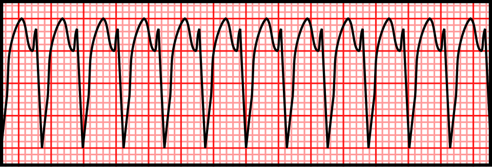
      Published vector teaching illustration of monomorphic ventricular tachycardia, with repeated broad complexes
      Regular + monomorphic ≠ SVT.

      Left: original conceptual timing diagram, CC BY 4.0 or MIT. Right: Rocuronium Bromide, Wikimedia Commons · CC0 1.0. Unchanged PNG rendering of the source vector. Teaching illustration, not a patient recording.

      Case A · positive early step

      Stable regular WCT; clear RS in V3; longest onset-to-S-nadir 120 ms. Brugada stops at step 2 and favors VT. A normal-looking V1 does not veto that result. Recheck the measurement, compare baseline ECG, and follow the appropriate WCT treatment pathway.

      Case B · conflicting morphology

      Young adult, regular RBBB-like WCT with a superior axis and brisk initial forces. Typical rsR′ or an aVR ratio >1 does not exclude fascicular VT. Document the discordant clues and obtain expert review rather than selecting whichever algorithm says SVT.

      Case C · wrong population

      Very rapid irregular WCT with changing QRS width and shape: suspect pre-excited AF among the differential. Stop regular-WCT scoring. Avoid A–V nodal blockade; manage the rhythm and hemodynamics urgently. A regular pre-excited tachycardia can also mimic slow ventricular activation and produce false-positive VT criteria.

      What independent validation changes

      In the 260-WCT head-to-head study, reference diagnoses came from EPS (216), device electrograms (38) and serial ECGs (6). Brugada accuracy was 77.5%; RWPT-II accuracy 68.8%. These data argue against treating derivation accuracy as universal or averaging algorithm outputs into a new diagnosis.

      Capture/fusion must be physiologically plausible, not simply a narrow or different-looking beat. Artifact, intermittent aberrancy, pacing and ectopy can confuse the pattern. Lack of demonstrable A–V dissociation is common in VT; its absence is not a negative mechanistic test.

      Report example: “Regular monomorphic WCT. VT favored by prolonged precordial RS interval; atrial activity indeterminate. Baseline tracing unavailable. Manage as uncertain/likely ventricular WCT pending expert assessment.” Separate what was measured from what was inferred.

      Check your reasoning: Two algorithms favor SVT but clinical and morphologic concern for VT remains. What should the report say?

      State the observed measurements, the algorithm classifications and the remaining uncertainty. Do not manufacture consensus probabilities; use a management pathway safe for possible VT and seek expert assessment.

      QT ends with T; a separate U is excluded

      Left: QRS onset. Center: T wave. Small wave at right: separate U, excluded.
      Dashed bracket: QT to the tangent–baseline intersection. Lower solid bracket: QT to the later threshold endpoint. Original schematic; not a patient tracing or calibrated waveform · CC BY 4.0.
      1. Choose and document. Inspect all leads; use one with a clear terminal T, often II or V5/V6. Record lead, speed, gain, beat selection and endpoint method. Follow the same method on serial ECGs.
      2. Mark QRS onset. Start at the beginning of ventricular depolarization, including an initial Q if present, rather than the R peak.
      3. Mark terminal T. Threshold measurement follows T to the baseline. The tangent method extends the steepest terminal downslope to the isoelectric baseline. In a negative T, use the terminal return toward baseline. A second component of a genuinely biphasic/notched T belongs to T; a separate U does not.
      4. Check another lead. T–U fusion, low amplitude and noise can make the endpoint indeterminate. Do not silently measure QU or invent precision: compare leads and obtain expert review if the decision hinges on it.
      Methods are not interchangeable. In a trained-reader study, tangent measurements were generally shorter than threshold measurements. A change of method can resemble a biological QT change.

      For stable sinus rhythm, use several representative beats. In AF, do not cherry-pick a single short or long cycle: a multiple-beat average better matched subsequent sinus-rhythm measurements in a comparative study. No universal AF measurement/correction method is established; document the averaging approach and residual uncertainty.

      Check your reasoning: An apparent QT prolongation disappears when a separate U wave is excluded. What should be reported?

      Report the measured QT, the lead and endpoint method, and any unresolved T–U ambiguity. QU is not interchangeable with QT.

      Bazett

      QTcB = QT / √RR

      Usually inflates QTc during tachycardia and can undercorrect at slow rates.

      Fridericia

      QTcF = QT / ∛RR

      Often has less rate dependence; it is still a population correction, not an individual truth.

      Use RR in seconds. QT may remain in milliseconds, giving QTc in milliseconds. State the method; a machine’s “QTc” without its formula is incomplete information.

      Arithmetic exercise, not a patientQTcBQTcF
      QT 400 ms; RR 0.60 s (100/min)516 ms474 ms
      QT 480 ms; RR 1.50 s (40/min)392 ms419 ms
      QT 440 ms; RR 1.00 s (60/min)440 ms440 ms
      1. Measure first. Verify the endpoint and QRS width before interpreting a computed QTc.
      2. Choose for the question. A congenital-LQTS diagnostic score uses its specified correction; do not quietly replace it with another formula. Drug-specific initiation protocols may likewise prescribe a method.
      3. Compare consistently. Use the same lead, method and correction longitudinally. Reassess after a stable rate when feasible.
      QT adapts with a delay. Abrupt rate changes produce QT/RR hysteresis; the immediately preceding RR may not represent the rate history governing the T wave. Neither formula fixes that problem.

      In a large observational study, Fridericia reduced rate dependence relative to Bazett in recordings without conduction defects or ventricular pacing. This supports deliberate formula choice, not switching formulas until a desired threshold is crossed.

      Check your reasoning: At QT 400 ms and RR 0.60 s, why is QTcB about 516 ms while QTcF is 474 ms?

      The square-root and cube-root corrections diverge at fast rates. Recheck the measurement and clinical context; neither number alone proves or excludes a dangerous repolarization disorder.

      QT = QRS + JT
      JT = QT − QRS

      A bundle-branch block lengthens ventricular activation and therefore QT. A conventional narrow-QRS QTc cutoff cannot simply identify how much of that increase is abnormal recovery. Report rhythm, QRS width, raw QT, rate and the chosen adjustment.

      1. Establish the context. Compare a prior narrow-QRS ECG when available. New conduction disease also needs its own explanation.
      2. Inspect repolarization separately. AHA/ACCF/HRS guidance favors JT assessment in conduction delay. State exactly how any rate correction is performed: “JTc” may mean a rate-corrected JT or QTc minus QRS, which are not algebraically identical.
      3. If using an LBBB estimate, name it. The simplified Bogossian approach is QTm = measured QT − 0.50 × QRS. Subtract half of the full LBBB QRS duration before heart-rate correction, not half of only the excess above 120 ms.

      Arithmetic exercise: LBBB, 60/min

      QT 520 ms; QRS 160 ms → JT 360 ms; QTm 440 ms. At RR 1.00 s, Bazett and Fridericia leave QTm at 440 ms. This illustrates decomposition; it is not an assurance of drug safety.

      Validation boundary. The original 60-person pacing experiment estimated 48.5% of QRS; the practical 50% form was subsequently evaluated in intermittent and post-TAVI LBBB. It is an estimate, not a universal validated correction for every paced rhythm, RBBB, nonspecific delay or rate. Do not silently generalize it or apply congenital-LQTS scoring thresholds to QTm.

      No universal JTc threshold is supplied here. A borderline estimate with syncope, T–U distortion or ventricular ectopy needs expert interpretation rather than a second decimal place.

      Check your reasoning: For LBBB QRS 160 ms, how much does the simplified Bogossian method subtract from raw QT?

      80 ms, half of the full QRS duration, before rate correction. Its limited validation does not make the result a universal torsades-risk cutoff.

      1. Recognize the substrate. QT prolongation plus reduced repolarization reserve: QT-active drugs or interacting drugs, low potassium/magnesium, bradycardia/pauses, and impaired drug clearance.
      2. Recognize the trigger. A premature beat may be followed by a long pause; the next beat develops exaggerated T–U prolongation. A subsequent early ventricular beat can initiate polymorphic VT: the classic short–long–short sequence.
      3. Escalate the warning. QTc >500 ms or an increase ≥60 ms after an at-risk drug warrants prompt review, especially with post-pause distortion, alternans, couplets or nonsustained polymorphic VT. These are warning thresholds, not a claim that every prolonged QT causes torsades.
      4. Act on the setting. Stop the culprit when appropriate, review interactions and clearance, correct electrolytes and provide monitored care with immediate defibrillation available. Recurrent pause-dependent episodes may require rate support under specialist direction.

      Torsades with prolonged QT

      Magnesium is used even when its serum value is normal. Prevent recurrent bradycardia/pauses; address the cause.

      Polymorphic VT with normal QT

      Do not automatically call it torsades. Acute ischemia and other mechanisms require a different evaluation.

      Sustained polymorphic VT or VF is an emergency. Use immediate resuscitation and defibrillation according to the clinical rhythm. Do not delay treatment while measuring QT.

      Drug decisions also depend on the agent and clinical benefit: follow its specific monitoring protocol. Rate acceleration with drugs is not a generic maneuver for congenital LQTS; obtain expert help. A prior “normal” ECG does not eliminate an acquired multi-hit risk.

      Check your reasoning: What makes a post-pause beat with striking T–U distortion and new ventricular couplets concerning?

      It is a warning pattern for pause-dependent torsades in the appropriate long-QT setting, prompting urgent cause reversal and monitored escalation before sustained arrhythmia.

      1. Exclude an acquired explanation. Recheck QT manually and review drugs, electrolytes, bradycardia and conduction delay. A reversible cause and an inherited predisposition can coexist.
      2. Apply the stated criteria. ESC 2022 supports diagnosis with QTc ≥480 ms on repeated 12-lead ECGs or a modified diagnostic score >3; a pathogenic mutation establishes diagnosis regardless of QT duration. In arrhythmic syncope or cardiac arrest, QTc ≥460 ms raises a stronger diagnostic concern.
      3. Escalate appropriately. Use inherited-arrhythmia assessment and genetic counseling, including family evaluation. A variant of uncertain significance is not interchangeable with a pathogenic variant.

      Modified score: key weights

      FindingPoints
      Resting QTc ≥480 / 460–479 / male 450–459 ms3.5 / 2 / 1
      QTc ≥480 ms at fourth minute of recovery1
      Torsades / T-wave alternans / notches in 3 leads2 / 1 / 1
      Low heart rate for age0.5
      Syncope with stress / without stress2 / 1
      Definite family LQTS / unexplained first-degree SCD <301 / 0.5
      Pathogenic mutation3.5
      Use the whole defined score, not a points scavenger hunt. Resting QT categories are alternatives. Clinical events and family findings require correct attribution; avoid double-counting the same event/person. The conventional score uses Bazett QTc and applies without secondary QT-prolonging causes.

      A low or borderline resting QTc does not exclude concealed familial LQTS. Conversely, a borderline machine value without corroborating evidence is not sufficient to attach a lifelong inherited diagnosis.

      Check your reasoning: Does a normal resting QTc exclude LQTS in a relative from a family with a pathogenic LQTS variant?

      No. Reduced penetrance can conceal the resting ECG phenotype; targeted family/genetic assessment is needed.

      LQT1 clue: broad base

      A broad T-wave base is an association, not a genotype diagnosis.

      LQT2 clue: low or notched

      Two low peaks illustrate a bifid or notched T wave.

      LQT3 clue: late onset

      A long flat segment precedes the late T wave.

      Original schematics; not patient tracings or calibrated waveforms · CC BY 4.0.

      LQT1 association

      Broad-based, prolonged T waves can accompany KCNQ1-related disease.

      LQT2 association

      Low-amplitude or bifid/notched T waves can accompany KCNH2-related disease.

      LQT3 association

      A long relatively isoelectric ST interval followed by a late T can accompany SCN5A-related disease.

      These are group associations from genotype–phenotype studies. There is substantial overlap and variation across leads, rate and serial ECGs. Morphology can direct scrutiny and family evaluation; it cannot establish a genotype or choose a genotype-specific treatment on its own. Normal-looking T waves do not exclude a pathogenic variant.

      Use recovery deliberately

      1. Specify the test. Obtain supervised exercise and recovery recordings when appropriate to the inherited-arrhythmia evaluation.
      2. Keep the clock. QTc ≥480 ms at the fourth minute of recovery adds one diagnostic-score point; it is not interchangeable with a peak-exercise or immediate-recovery value.
      3. Keep the population in mind. The exercise-algorithm derivation/validation study evaluated relatives of LQTS probands, not indiscriminate low-risk population screening.
      A recovery value is one piece of evidence. Interpret its endpoint, formula, medications and pretest probability; do not diagnose LQTS from a single noisy post-exercise beat.
      Check your reasoning: Can a bifid T wave establish LQT2?

      No. It is an associated morphology with overlap; diagnosis and genotype require the complete clinical and genetic evaluation.

      Type 1: coved

      The elevated coved segment descends into a negative T wave. Apply the lead, amplitude and clinical criteria below.

      Type 2: saddleback

      A raised saddleback segment with an upright T wave. Type 2 morphology is not diagnostic alone.

      Original schematics; not patient tracings or calibrated waveforms · CC BY 4.0.

      Type 1 morphology

      J-point/ST elevation ≥2 mm (0.2 mV at standard gain) with a coved descending ST segment followed by a negative T wave in at least one of V1 or V2, recorded in the second, third or fourth intercostal space. Confirm the J point at QRS end; the 2025 provocation criteria require the pattern in at least two beats.

      Type 2 morphology

      A saddleback right-precordial ST configuration is suggestive but not diagnostic of Brugada syndrome. Benign rSr′ variants and lead-position effects can resemble it.

      1. Name what is present. Describe type 1 pattern, lead and electrode position. A simple rSr′ or right bundle-branch block label does not capture the diagnostic ST–T contour.
      2. Look for a mimic. Evaluate ischemia, electrolyte disorders and other reversible or structural explanations. Resolution after correction alone does not settle whether underlying susceptibility exists.
      3. Separate pattern from syndrome. A spontaneous type 1 pattern after exclusion of other heart disease has different diagnostic weight from an induced pattern. Drug-induced type 1 alone is less specific and requires supporting clinical/family/genetic evidence under contemporary guidance.
      Two unrelated uses of “Brugada.” The WCT algorithm distinguishes mechanisms of a broad-complex tachycardia. It does not diagnose the inherited Brugada syndrome, and a type 1 resting pattern does not identify every future tachycardia mechanism.

      Risk assessment depends on documented ventricular arrhythmia, probable arrhythmic syncope, spontaneous versus induced pattern and the broader evaluation. The drawing is a contour lesson, not a calibrated diagnostic tracing.

      Check your reasoning: Is an isolated saddleback pattern sufficient to diagnose Brugada syndrome?

      No. Type 2 is nondiagnostic; verify lead placement, alternatives and clinical context, then obtain specialist assessment when indicated.

      Standard recording

      V1: fourth intercostal space, right sternal border.
      V2: fourth intercostal space, left sternal border.

      Intentional high-right recording

      Record V1/V2 additionally at the third and/or second intercostal spaces to sample the right ventricular outflow tract region. Label every position.

      1. Acquire a valid baseline. Accidental superior placement on a supposedly standard ECG creates ambiguity. Keep standard leads and intentional high-right recordings distinguishable.
      2. Record the circumstance. Document fever, relevant drugs, electrolytes and symptoms. The phenotype can be intermittent; compare serial recordings.
      3. Treat fever promptly. Fever can unmask the pattern and increase arrhythmic risk in susceptible people. Syncope, ventricular arrhythmia or high-risk presentation needs urgent assessment rather than waiting for an outpatient repeat.
      4. Use drug challenge selectively. Sodium-channel blocker testing belongs in an experienced, monitored setting with resuscitation capability and a predefined protocol. It can produce conduction slowing and ventricular arrhythmia, and a positive test has imperfect specificity.
      Do not challenge every saddleback ECG. The 2025 multisociety consensus does not advise routine provocation for an asymptomatic type 2/3 pattern without a supportive family history. Test selection changes the meaning of a positive result.

      Review possible Brugada-provoking drugs with a reliable, current specialist resource; do not use this chapter as a drug list. A fever- or drug-associated pattern should be reported with its trigger and expert interpretation. “It disappeared” describes a dynamic phenotype; it does not by itself prove a harmless phenocopy or establish an inherited syndrome.

      Check your reasoning: Why must a high V1/V2 recording be explicitly labeled?

      Second/third-space placement intentionally changes the sampled region. Without labeling, it can be mistaken for a standard recording or an acquisition error and mislead serial interpretation.

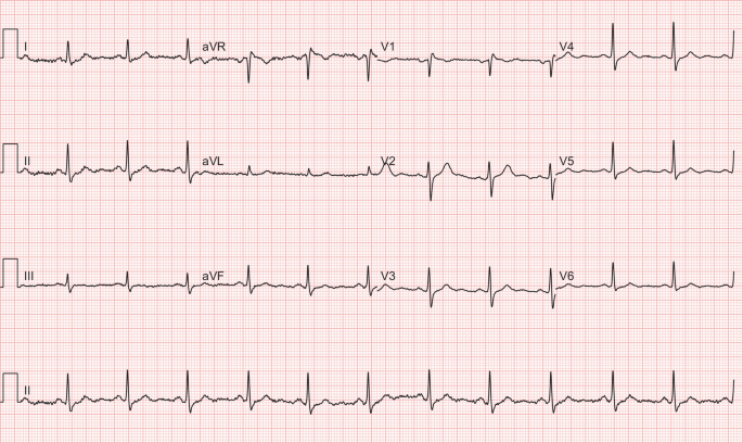
      This published case pairs an initial ECG during fever with a repeat after fever resolved. The authors described a type 1-like pattern in V1 on the first recording. These are original clinical images, not generated or redrawn signals.

      Overview only: open each unchanged image to inspect the right-precordial contour and calibration at full resolution.
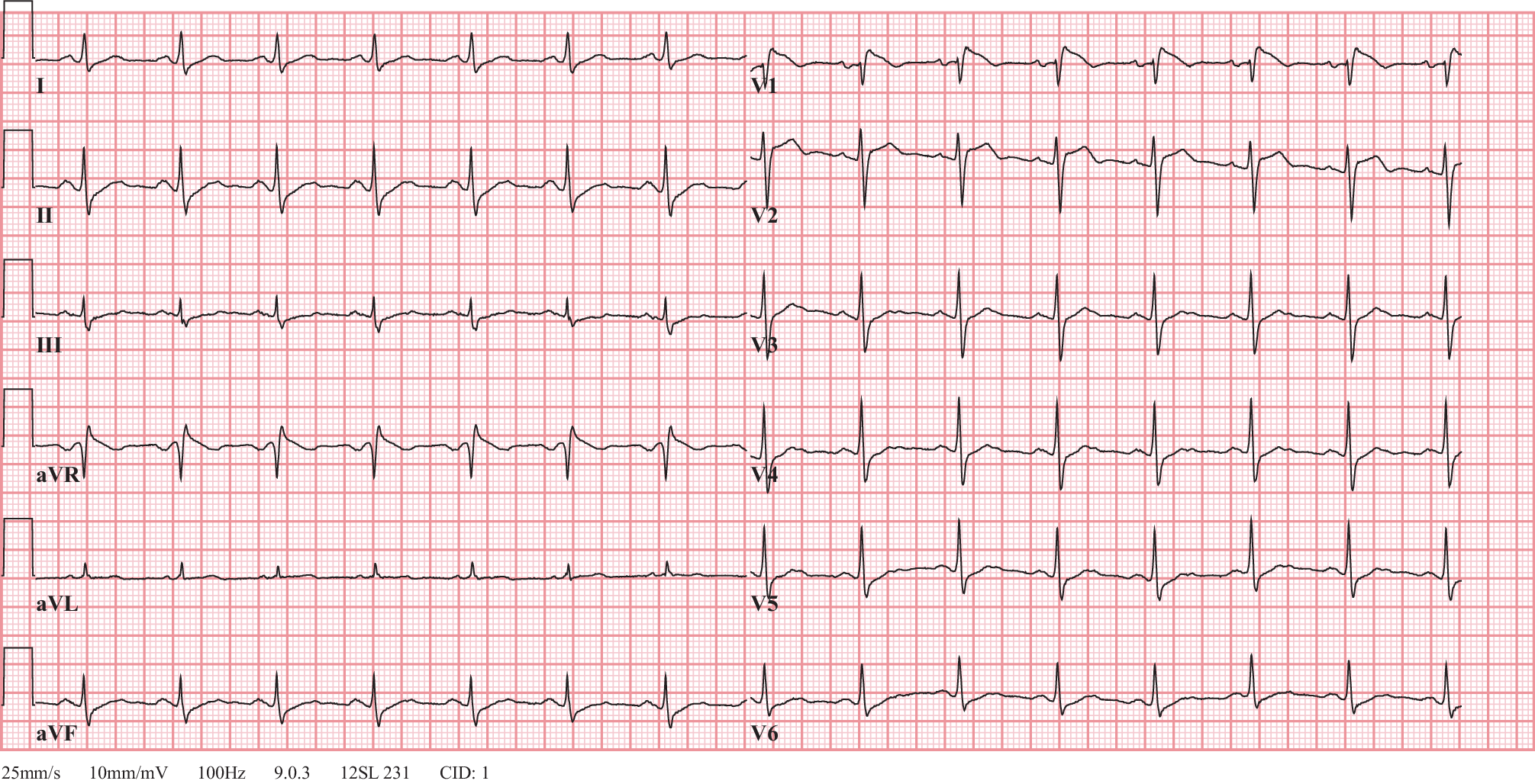
      Published figure 1: 12-lead ECG with fever-associated coved right-precordial pattern in V1
      Fever · source Figure 1. van de Poll and van der Werf, 2020 · CC BY 4.0 · reproduced unchanged.
      Published figure 2: repeat ECG after fever resolution with resolution of the reported Brugada-like pattern
      Recovery · source Figure 2. van de Poll and van der Werf, 2020 · CC BY 4.0 · reproduced unchanged.
      1. Find V1 before comparing. The two figures use different lead layouts and recording rates; follow the labels instead of assuming the same panel position.
      2. Compare contour. Examine the terminal QRS, elevated ST segment and subsequent T, not just the height of one peak.
      3. Read the clinical provenance. The report’s first subject had no reported syncope or relevant family history, no observed arrhythmia during admission, and resolution of the pattern after fever treatment. Follow-up including genetic testing was planned.
      4. Keep the limit. Planned testing is not a confirmed genetic result. This paired example demonstrates dynamic expression; it does not prove that all fever-associated patterns are benign or that this individual had genetically confirmed inherited Brugada syndrome.
      Interpretation exercise: “Fever-associated right-precordial type 1-like pattern, resolving on the subsequent source ECG; clinical and inherited-arrhythmia evaluation remain essential.”
      Check your reasoning: What can this real before/after pair establish without inventing follow-up?

      It demonstrates the reported fever-associated ECG change and subsequent resolution. It cannot establish an unpublished genotype, long-term outcome or universal risk rule.

      Sokolow–Lyon

      S in V1 + larger R in V5 or V6 ≥35 mm at 10 mm/mV.

      Cornell voltage

      R in aVL + S in V3 >28 mm in men or >20 mm in women at 10 mm/mV.

      1. Check gain. The authentic example in the next case uses 5 mm/mV: double measured millimeters to compare with standard-gain thresholds, or calculate in mV directly.
      2. Measure named deflections. Sum amplitudes relative to the local baseline, not total peak-to-peak QRS height.
      3. Look beyond voltage. Lateral downsloping ST depression with asymmetric T inversion can be secondary to altered activation/repolarization. Report the pattern and compare prior tracings.
      4. Correlate anatomy. Echocardiography assesses mass, geometry and competing disease when clinically indicated.

      Voltage criteria are insensitive and depend on age, body habitus, sex, ancestry and lead placement. Thin or athletic people can have large voltages; obesity or emphysema can attenuate them. Bundle block, pacing and scar complicate standard criteria. “Strain” is a conventional ECG description, not a measurement of myocardial deformation. A broad/notched P in II or prominent terminal negative P component in V1 suggests left atrial abnormality; tall inferior P waves suggest right atrial abnormality. Confirm chamber size by imaging rather than equating electrical criteria with enlargement.

      Worked case. S(V1) 22 mm + R(V5) 18 mm at standard gain totals 40 mm: positive Sokolow–Lyon voltage. That calculation does not identify the cause of LVH or prove that coexisting chest pain is nonischemic.
      Do not overcall. A normal-voltage ECG does not exclude anatomical LVH; secondary ST–T changes do not exclude superimposed ischemia.
      Check your reasoning: At 5 mm/mV, S(V1) + R(V5) measures 20 mm. What is the standard-gain equivalent?

      40 mm at 10 mm/mV, equivalent to 4 mV. This exceeds the Sokolow–Lyon threshold but is not an anatomical diagnosis by itself.
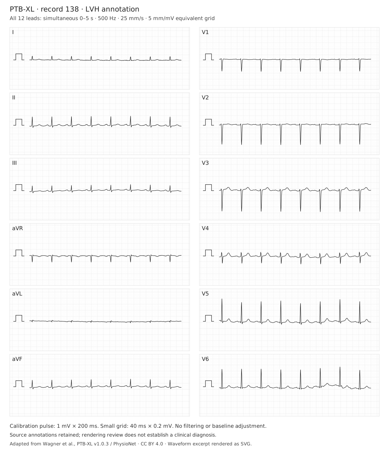
      Authentic PTB-XL record 00138, source annotation LVH; open full tracing for calibrated measurement.
      Wagner et al., PTB-XL v1.0.3, record 00138: LVH (dataset annotation). Simultaneous 0–5 s, 500 Hz, 25 mm/s, 5 mm/mV; amplitudes unchanged, no filtering. SVG rendering under CC BY 4.0. Source, transformations and checksums. Open full tracing; overview is not a substitute for measurement.
      Reading exercise. Before applying a voltage threshold, identify the gain and named leads. Measure S in V1 and the larger R in V5/V6 relative to their local baselines. Then examine aVL and V3 for Cornell voltage.

      This record is shown at half standard gain. Double measured millimeters before comparing with thresholds stated at 10 mm/mV, or work directly in mV. Inspect lateral ST–T morphology and the atrial waveform separately. The dataset annotation does not establish the anatomical cause, exclude ischemia, or require every voltage criterion to be positive.

      Check your reasoning: Why can a sum below 35 mm in this image still satisfy standard-gain Sokolow–Lyon voltage?

      The displayed gain is 5 mm/mV. A measured sum of 17.5 mm corresponds to 3.5 mV, or 35 mm at standard 10 mm/mV gain. Apply the threshold only after checking calibration and measuring the correct deflections.

      Chronic rightward forces

      Right axis, a dominant R in V1 and persistent lateral S waves may support RVH in context. Dominant R in V1 also has other causes.

      Acute RV stress

      New right-precordial T inversion, RBBB or S1Q3T3 can accompany acute PE, but are neither required nor diagnostic.

      1. Validate the recording. Recheck V1 placement, QRS duration and comparison ECG.
      2. Describe the components. Axis, R/S distribution, conduction and ST–T findings are separate observations.
      3. Use the time course. Chronic pulmonary or congenital disease differs from sudden dyspnea, syncope or hypoxemia.
      4. Use the clinical pathway. Assess PE probability and obtain indicated testing; imaging evaluates RV structure/function.

      In a community population without clinical cardiovascular disease, the MESA-RV study found ECG criteria unsuitable for screening mild RVH. Performance in selected congenital or pulmonary-hypertension populations cannot be transplanted to an incidental ECG. The source-annotated RVH record in the next case is a comparison exercise, not proof that every voltage criterion must be present.

      Worked case. Sudden dyspnea with new V1–V4 T inversion raises concern for acute RV stress. A tracing without S1Q3T3 would not safely lower that concern enough to stop the PE evaluation.
      Do not overcall. Do not label a generic notched inferior R wave “RV strain.” Crochetage has a different association, developed in the next chapter.
      Check your reasoning: Can an ECG without RV strain exclude pulmonary embolism?

      No. Clinical probability and the recommended diagnostic pathway govern PE assessment; ECG is complementary.
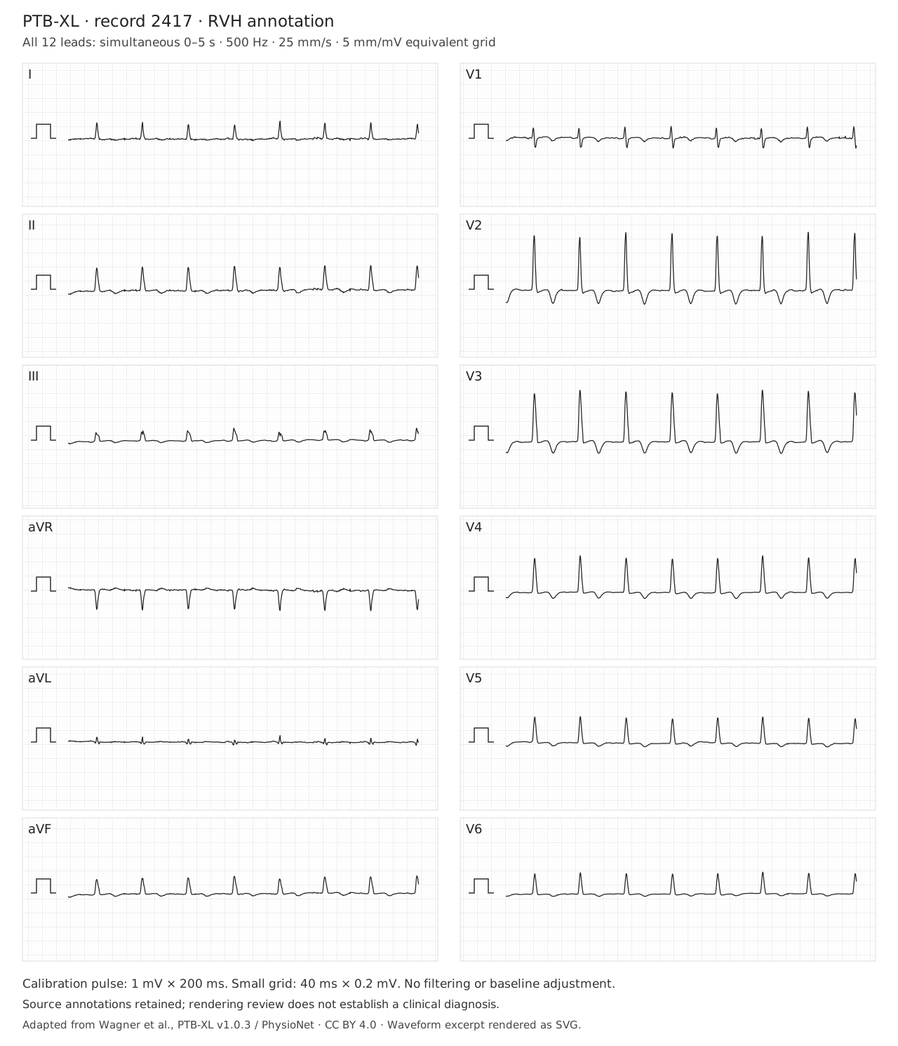
      Authentic PTB-XL record 02417, source annotation RVH; open full tracing for calibrated measurement.
      Wagner et al., PTB-XL v1.0.3, record 02417: RVH (dataset annotation). Simultaneous 0–5 s, 500 Hz, 25 mm/s, 5 mm/mV; amplitudes unchanged, no filtering. SVG rendering under CC BY 4.0. Source, transformations and checksums. Open full tracing; overview is not a substitute for measurement.
      Reading exercise. Inspect limb-lead polarity, QRS duration, the R/S relationship in V1, lateral S waves and right-precordial repolarization. Record these observations separately before comparing them with the source annotation.

      The displayed gain is 5 mm/mV; use the calibration pulse for amplitude measurements. The RVH label is a dataset annotation, not independent confirmation of RV size or pressure. A dominant R in V1 has competing explanations. Compare a prior ECG and correlate clinical context and imaging. This tracing cannot establish acute pulmonary embolism or safely exclude it.

      Check your reasoning: Does the RVH annotation establish acute RV strain or pulmonary embolism?

      No. The source annotation describes a dataset label. Describe the ECG findings, assess time course and clinical probability, and use indicated testing. Neither RVH voltage criteria nor their absence diagnose or exclude acute PE.

      Inferior lead: crochetage

      Schematic inferior R wave with a notch near its ascent and apex
      Notch near the R-wave ascent or apex. Original schematic; not a recorded ECG.

      Right precordial lead: rSr′

      Schematic right precordial rSr prime; the terminal R prime differs from crochetage
      Terminal R′ is a different feature. Original schematic; not a recorded ECG.

      Crochetage describes notching near the ascent or apex of the R wave in inferior leads II, III and aVF. Its classic association is secundum atrial septal defect. Do not use the term interchangeably with terminal R′ in V1 or with every fragmented QRS pattern.

      1. Confirm the notch is real. Look for reproducibility across beats and at diagnostic bandwidth; noise and processing can create or erase fine detail.
      2. Check all inferior leads. Note whether the feature occurs in one, two or all three; distribution mattered in the original study.
      3. Assemble the context. Consider accompanying rightward axis, incomplete RBBB and clinical evidence of right-sided volume loading, without treating any as proof.
      4. Resolve anatomy. Echocardiography evaluates septal anatomy and right-heart size; further shunt assessment follows the clinical question.

      Heller and colleagues compared 1,560 people across several structural diagnoses and controls. Crochetage occurred in 73.1% of the secundum-ASD group, but also in other groups. Presence in all three inferior leads was more specific in that study. These selected-population results are not a universal screening probability.

      Worked case. A reproducible notch near R peaks in II, III and aVF accompanies an rSr′ in V1 and an unexplained systolic flow murmur. The useful next inference is “evaluate for a shunt,” not “the ECG proves ASD.”
      Do not overcall. The original schematic teaches shape; no acquired patient tracing or validated diagnostic sensitivity is implied by it.
      Check your reasoning: What is the classic structural association of inferior-lead crochetage?

      Secundum ASD. It is not a specific generic marker of acute RV strain, and imaging is needed to establish anatomy.
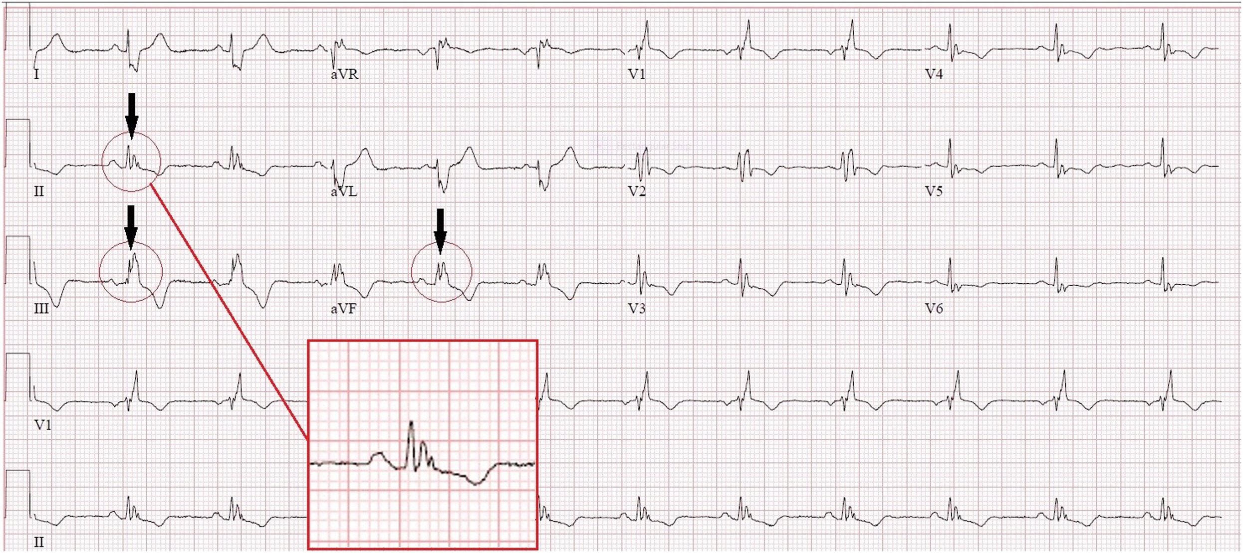
      PUBLISHED ECG / SECUNDUM ASDFind the notch near the R-wave apex in the inferior leads.
      Complete published ECG from Zeman et al., Crochet Leads the Way, Figure 2, with original arrows, circles and inset showing inferior-lead crochetage.
      Zeman et al. (2023), Figure 2, Crochet Leads the Way, JACC: Case Reports. © 2023 The Authors; Elsevier/ACC. Original authors’ arrows, circles and inset retained. Original article. Reproduced unchanged under CC BY-NC-ND 4.0. Noncommercial reuse only; no distribution of modified versions. This third-party figure is excluded from the guide’s general license. Open the complete figure at full resolution.
      1. Locate the notch within the QRS.

        Use the authors’ magnified inset and compare the inferior leads. The sign is a notch near the R-wave summit, not simply any terminal R′.

      2. Keep the association specific.

        Crochetage is associated with secundum atrial septal defect. It is not a generic marker of RV strain or a diagnostic criterion for PE.

      3. Separate illustration from validation.

        This published case shows the morphology. The diagnostic-performance evidence comes from the separate Heller cohort cited in the preceding chapter.

      What the image should trigger: a focused examination and appropriate structural evaluation when the overall findings suggest a shunt. The notch alone does not establish the anatomy or hemodynamic significance.
      Check your reasoning: What does this published crochetage tracing establish by itself?

      It illustrates the characteristic morphology in one source case. It does not establish sensitivity, specificity, shunt size or an anatomical diagnosis in a different patient.

      Voltage alone

      Illustrative low-amplitude QRS; uncalibrated conceptual waveform
      Low signal has multiple possible causes. Original schematic, not calibrated patient data.

      Voltage + imaging + phenotype

      • Unexpectedly thick ventricular walls.
      • Relatively small QRS amplitudes.
      • Conduction disease or extracardiac clues.

      Investigate an infiltrative process when the combined findings warrant it.

      Conventional low-voltage thresholds are QRS peak-to-peak amplitudes ≤5 mm in every limb lead or ≤10 mm in every precordial lead at 10 mm/mV. State which distribution is involved; one small lead does not meet a global criterion. First exclude reduced gain, poor contact and acquisition differences.

      1. Verify the amplitude. Use the calibration pulse and all relevant leads; compare a prior recording at the same gain.
      2. Consider attenuation. Body habitus, emphysema, effusions and other extracardiac factors may reduce the measured signal.
      3. Compare imaging. Increased wall thickness with unexpectedly low or modest voltage raises suspicion for amyloidosis, especially with conduction disease or a pseudoinfarction pattern.
      4. Follow the disease pathway. Integrate echocardiography/CMR, phenotype and appropriate amyloid testing rather than typing the disease from ECG.

      Normal or high QRS voltage does not exclude cardiac amyloidosis; the classic voltage–thickness mismatch is absent in many affected patients. Low voltage also cannot distinguish AL from ATTR. A positive bone-tracer scan should not be interpreted as ATTR without the required monoclonal-protein assessment.

      Worked case. An adult has 16-mm ventricular walls, heart-failure symptoms, conduction delay and only modest limb voltages. The mismatch is a reason to investigate, even if the strict low-voltage cutoff is not crossed.
      Do not overcall. Neither low voltage nor a pseudoinfarction pattern proves amyloid. Conversely, a voltage-positive LVH ECG is not a reason to dismiss otherwise convincing infiltrative clues.
      Check your reasoning: Must the strict low-voltage threshold be met to suspect amyloidosis?

      No. Relative voltage–wall-thickness discordance and the broader phenotype matter; normal voltage does not exclude disease.

      Capture

      Pacing stimulus precedes a paced QRS
      Stimulus activates myocardium. Original conceptual strip.

      Fusion

      Pacing stimulus precedes a QRS reflecting paced and native activation
      Paced and native activation both contribute. Original conceptual strip.

      Pseudofusion

      Stimulus coincides with native QRS without contributing to activation
      Spike without material QRS contribution. Original conceptual strip.
      1. Establish timing. Identify atrial activity, stimulus markers, native QRS complexes and their relationships. Digital display artifacts are not always true pacing stimuli.
      2. Assess capture. A stimulus should produce the expected atrial or ventricular response when tissue is excitable. Compare morphology across multiple beats.
      3. Recognize mixed activation. Fusion combines paced and intrinsic activation; pseudofusion is a pacing stimulus that does not contribute materially to an already activated QRS.
      4. Use the device record. New pauses, symptoms or changing paced morphology require clinical assessment and interrogation, not a diagnosis from one printed strip alone.

      Conventional RV pacing often resembles LBBB, but pacing site, conduction-system capture, biventricular pacing and fusion can produce other morphologies. A relatively narrow QRS does not exclude pacing. Bipolar pacing spikes may be very small or filtered out; absence of a printed spike is not proof of absent output.

      CRT may deliberately exploit fusion with intrinsic conduction. Therefore an intermediate QRS shape is not automatically malfunction. Conversely, a pacing spike that falls in refractory tissue does not demonstrate successful capture simply because a QRS is nearby. Verify the interval and morphology.

      Worked case. A patient with CRT has alternating QRS shapes at similar rates. Compare the timing of intrinsic conduction and stimuli, then interrogate the device; do not call all changed beats PVCs or assume lead failure.
      Do not overcall. Secondary ST–T changes from pacing complicate ischemia interpretation. Use the dedicated ischemia framework and clinical context; do not declare the ECG uninterpretable or reassuring by default.
      Check your reasoning: Does a narrow QRS rule out ventricular pacing?

      No. Conduction-system pacing, fusion and some resynchronization configurations can produce relatively narrow complexes.

      Frequency ≠ heart rate

      Illustrative spectrum: dominant 95 Hz peak with shaded zero to 40 Hz bandwidth04095150Hz
      Original conceptual spectrum. Shading marks 0–40 Hz, not a simulated filter response.

      5700 rpm ÷ 60 = 95 Hz

      The observed interference frequency reflects rotation, not ventricular rate.

      A 40-Hz low-pass view retains less bandwidth and may clarify rhythm while removing important QRS detail.

      LVAD electromagnetic interference can obscure P waves, QRS boundaries and the baseline. Evaluate the patient and circulation immediately if unstable; neither apparent artifact nor a weak/absent palpable pulse establishes the rhythm in continuous-flow support.

      1. Improve contact first. Prepare skin, replace loose electrodes, support cables and reduce motion. Verify standard lead placement before comparing morphology.
      2. Compare simultaneously. Look for organized complexes in less affected leads and examine prior/device recordings. Record the LVAD model and prescribed speed as context.
      3. Preserve the diagnostic tracing. A documented 40-Hz low-pass view may clarify rhythm; retain the standard-bandwidth ECG for QRS/ST–T assessment. Targeted bandstop filtering needs appropriate technical support.
      4. Escalate uncertainty. Involve the VAD/electrophysiology team if rhythm or device behavior remains unclear. Never change pump speed for ECG acquisition.

      In a nine-patient study, HeartMate 3 at 5700 rpm produced a dominant 95-Hz artifact; model-specific spectra included additional peaks. Legacy HeartWare examples showed a dominant component near twice the rotational frequency. These observations explain interference; they are not validated noninvasive pump diagnostics.

      A 2024 electrode-placement study abstract found no alternative configuration that consistently reduced noise. Do not promise that a particular limb site, side of the body or manufacturer-specific arrangement will solve interference. If nonstandard placement is necessary, label it and avoid direct voltage/axis comparison with standard ECGs.

      Worked case. A 40-Hz view reveals regular ventricular complexes beneath dense noise. That answers a rhythm question; it does not certify preserved pacing spikes, QRS notches or ischemia-sensitive morphology.
      Check your reasoning: Should pump speed be changed to obtain a cleaner ECG?

      No. Optimize acquisition and documented ECG filtering, retain diagnostic bandwidth and involve the VAD team. Pump therapy is not an ECG acquisition control.
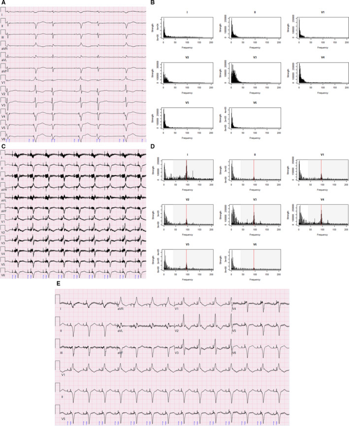
      PUBLISHED ECG / HEARTMATE 3Follow A/B before implantation → C/D after implantation → E with a 40-Hz low-pass filter.
      Complete Figure 1 from Loring et al., showing pre-LVAD ECG and spectrum, post-LVAD interference and spectrum, and a 40-Hz low-pass filtered ECG.
      Loring et al. (2020), Figure 1, Reducing ECG Artifact From Left Ventricular Assist Device Electromagnetic Interference. © 2020 The Authors; JAHA/Wiley. Original article. Reproduced unchanged under CC BY-NC-ND 4.0. Noncommercial reuse only; no distribution of modified versions. This third-party figure is excluded from the guide’s general license. Open the complete figure at full resolution.
      Why the pattern changes: the source case shows a 95-Hz component at 5700 rpm. A 40-Hz low-pass filter improves the rhythm view while removing high-frequency information. A cleaner appearance does not establish diagnostic fidelity for ST segments, QRS notches or pacing spikes.
      Check your reasoning: Does the cleaner filtered panel replace a standard diagnostic ECG?

      No. Preserve the standard-bandwidth recording and document filtering. The source figure demonstrates a tradeoff in one case; it does not validate every interval or morphology measurement after filtering.

      Inferior

      II, III, aVF
      Look for reciprocal change in I/aVL. If RV involvement is suspected, add right-sided leads.

      Anterior / septal

      V1–V4
      Check the distribution, evolution and R-wave progression; repeat misplaced V1/V2 before inferring a fixed scar.

      Lateral

      I, aVL, V5–V6
      Interpret alongside inferior and precordial reciprocal findings.

      Posterior mirror

      V1–V3 depression + upright T / dominant R
      Obtain V7–V9 when posterior occlusion is suspected.

      1. Find the J point and compare with baseline.

        Check gain and QRS morphology, then inspect contiguous leads. New ST elevation in two contiguous leads supports a STEMI pattern when appropriate clinical context and exclusions are met.

      2. Apply the correct thresholds.

        Usually ≥1 mm; in V2–V3, ≥2 mm in men ≥40 years, ≥2.5 mm in younger men, and ≥1.5 mm in women. These standard thresholds assume no confounding LVH or bundle-branch block.

      3. Act on the entire presentation.

        Persistent ischemic symptoms, shock, dynamic changes or an occlusion-equivalent pattern warrant urgent expert assessment even without classic thresholds.

      Posterior leads: V7 left posterior axillary line, V8 left mid-scapular line and V9 left paraspinal border, all level with V6. Posterior ST elevation ≥0.5 mm supports the diagnosis in context. Use ≥1 mm in men <40 years. Record V3R/V4R early when RV infarction is suspected.
      Check your reasoning: What should anterior ST depression with a posterior mirror pattern prompt?

      Additional posterior leads and prompt clinical reassessment for coronary occlusion, rather than treating every ST-depression pattern as the same risk category.

      STE +3 mm; S −20 mm

      3 / 20 = 15%. Elevation is small relative to the opposing S-wave depth.

      STE +3 mm; S −8 mm

      3 / 8 = 37.5%. The proportional criterion is met. Baseline and J-point elevation are the same as in the first panel.

      Original teaching schematics, not patient recordings. CC BY 4.0 or MIT. Timing and voltage are illustrative unless explicitly labeled.

      1 / Concordant elevation

      ST elevation ≥1 mm in a lead whose QRS is predominantly positive.

      2 / Concordant depression

      ST depression ≥1 mm in V1, V2 or V3.

      3 / Excessive discordance

      In a negative-QRS lead: J-point elevation ≥1 mm and at least 25% of the preceding S-wave depth.

      Any one positive criterion is concerning in the appropriate clinical presentation. Express the third as STE / |S| ≥0.25, or the signed ST/S ratio ≤−0.25.

      The original Sgarbossa rule scores concordant elevation 5 points, concordant V1–V3 depression 3, and discordant elevation ≥5 mm 2; a total ≥3 is positive. Do not mix the original score with the modified proportional rule.

      Check your reasoning: With 3 mm ST elevation above an 8 mm S wave, is the proportional criterion met?

      Yes: 3/8 = 0.375, above 0.25, and ST elevation is at least 1 mm. This is a positive modified criterion in a negative-QRS lead, interpreted within the clinical presentation.

      De Winter contour

      Upsloping J-point depression leads into a prominent T wave. Interpret with acute ischemic symptoms.

      Wellens: biphasic T

      Positive then negative anterior T wave; the clinical pattern often appears after pain resolves.

      Wellens: inverted T

      Deep symmetric anterior T inversion. Contour alone does not establish coronary anatomy.

      Original teaching schematics, not patient recordings. CC BY 4.0 or MIT. Timing and voltage are illustrative unless explicitly labeled.

      De Winter pattern

      Precordial upsloping J-point ST depression with tall, symmetric T waves in a patient with ischemic symptoms. The original series linked this to proximal LAD occlusion; do not treat the artery location as guaranteed in every case. With an acute ischemic presentation, obtain emergency coronary/reperfusion evaluation for immediate angiography.

      Wellens clinical pattern

      Recent angina with biphasic or deep symmetric anterior T-wave inversion, often when pain has resolved, without the expected Q-wave evolution. This is a high-risk presentation needing urgent cardiology assessment; avoid provoking ischemia with routine stress testing.

      Hyperacute versus hyperkalemic

      Broad, regional T waves with reciprocal/evolving changes favor ischemia; narrow peaked T waves may suggest potassium effects. Neither visual shortcut replaces symptoms, serial ECGs and laboratory assessment.

      Diffuse depression + aVR elevation

      Think widespread subendocardial ischemia or supply–demand imbalance. It does not uniquely identify acute left-main occlusion.

      Chest pain has stopped and V2–V3 now show deep symmetric T inversion. Is a pain-free patient “ruled out”?

      No. Interpret the preceding symptoms and ECG evolution. A Wellens-type clinical presentation remains high risk even between episodes.

      Check your reasoning: Why distinguish a Wellens pattern from an isolated inverted T wave?

      The syndrome requires clinical context and exclusion of important mimics. A T-wave shape alone cannot establish the coronary anatomy or urgency for every patient.

      Inspect the beginning of QRS

      The highlighted initial slur is the delta wave. Look for a coherent short-PR / delta / wider-QRS pattern across leads. Degree of fusion varies. Original uncalibrated schematic; CC BY 4.0 or MIT.
      1. Identify a coherent pattern.

        A short PR, delta wave and widened QRS support manifest ventricular pre-excitation. Fusion can make the pattern subtle; compare multiple leads and prior ECGs.

      2. Recognize the dangerous rhythm.

        A very fast, irregular wide-complex rhythm with changing QRS appearance may represent pre-excited AF. AV-nodal blocking drugs can be harmful; use urgent rhythm-specific management.

      3. Keep localization in its own validated framework.

        Initial delta-wave polarity, lead placement and the intended study population matter. A concealed pathway with no antegrade pre-excitation cannot be localized by a delta-wave algorithm.

      Check your reasoning: Why can a frontal QRS-axis angle not locate an accessory pathway?

      Mean QRS axis and initial delta-wave activation are different information. Fusion and anatomy prevent an unsupported one-angle-to-one-location mapping.

      REAL RECORD / PTB-XL 00003Describe the rhythm, axis and precordial progression and compare your reading with the source annotation below.

      Overview: open the full-resolution tracing to inspect intervals and morphology.
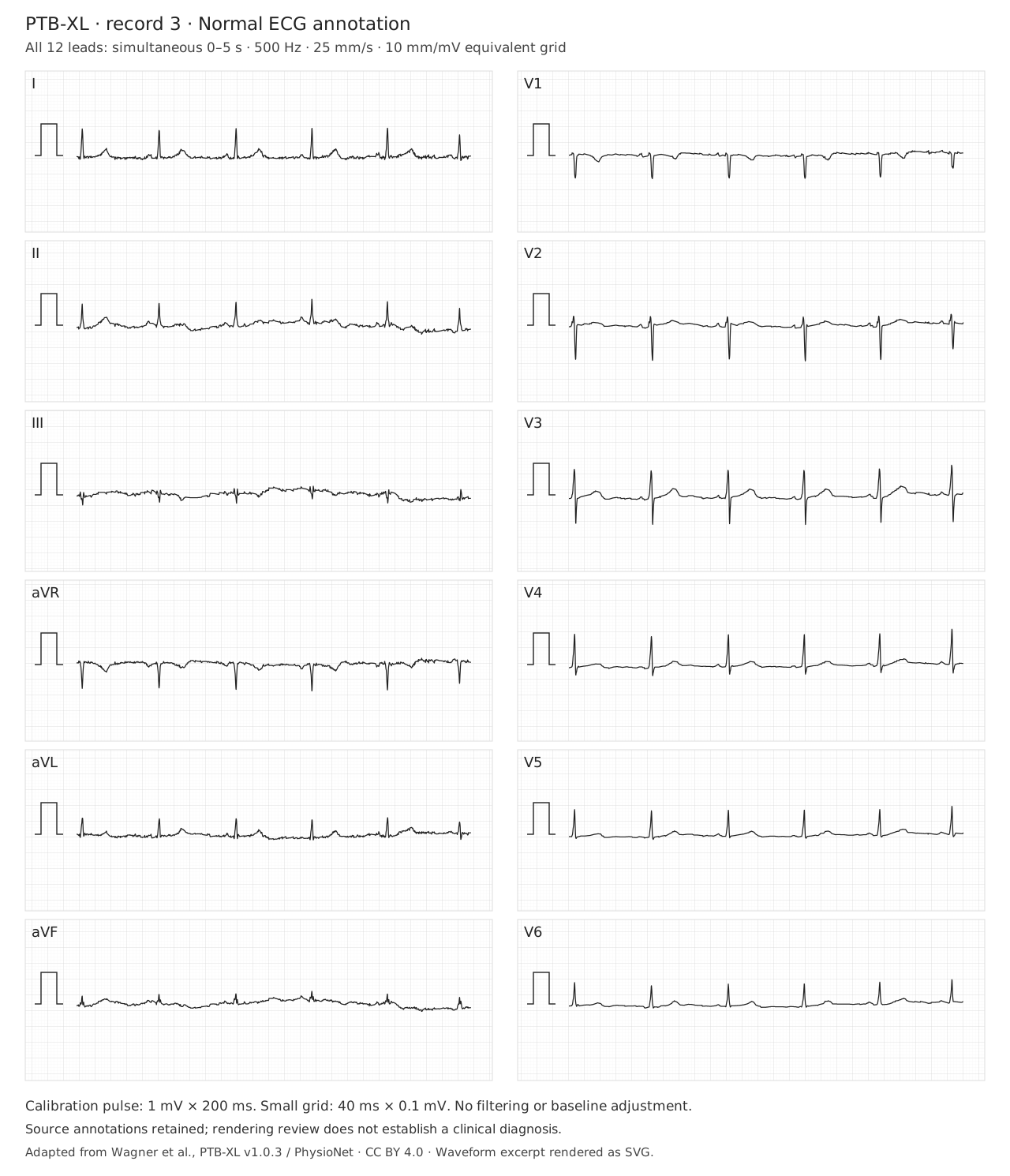
      Twelve simultaneous ECG leads from PTB-XL record 00003; source annotation NORM (normal ECG). Open full-size for calibrated inspection.
      PTB-XL v1.0.3 (version DOI), record 00003, source annotation: NORM (normal ECG). All 12 leads show the same 0–5 s interval at original 500 Hz. Grid: 25 mm/s and 10 mm/mV; use the depicted calibration after resizing. Wagner et al., PTB-XL; CC BY 4.0. Original dataset paper; PhysioNet platform. Original amplitudes retained. Open the full tracing · Attribution and transformations.
      Reveal the source annotation and the useful limits

      The dataset labels this record NORM (normal ECG) and SR. That is source metadata, not an independently adjudicated diagnosis or a statement that coronary disease is absent. Confirm the recording quality, atrial relationship, QRS width, axis and ST–T findings yourself.

      Three observations to practice: identify a reproducible atrial deflection; compare the signs of I, II and aVF; follow R-wave progression across V1–V6.
      Check your reasoning: Why keep both the source recording and its annotation?

      The recording supports independent inspection. The annotation provides dataset context, but must not substitute for reading the signal or establishing a clinical diagnosis.

      REAL RECORD / PTB-XL 00621Find the terminal forces in V1, I and V6. Then examine the repolarization pattern.

      Overview: open the full-resolution tracing to inspect intervals and morphology.
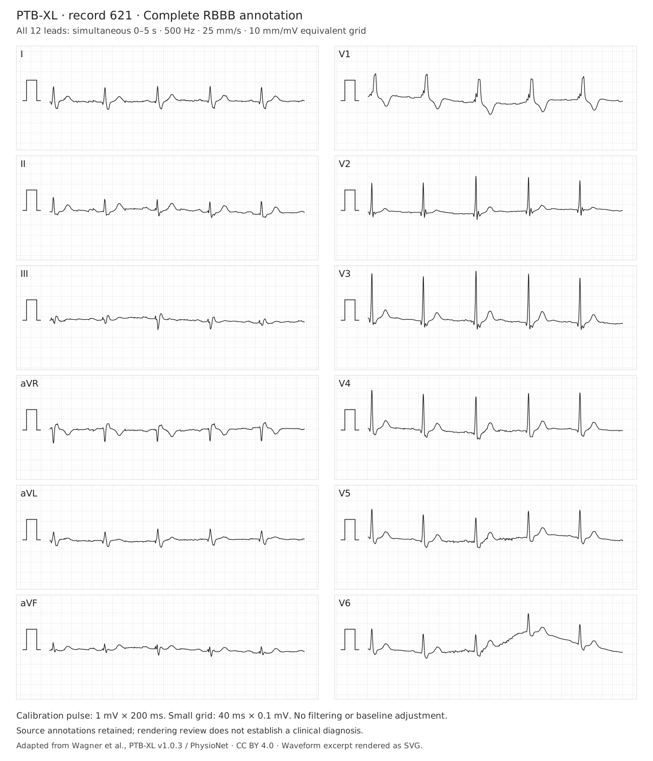
      Twelve simultaneous ECG leads from PTB-XL record 00621; source annotation CRBBB (complete right bundle branch block). Open full-size for calibrated inspection.
      PTB-XL v1.0.3 (version DOI), record 00621, source annotation: CRBBB (complete right bundle branch block). All 12 leads show the same 0–5 s interval at original 500 Hz. Grid: 25 mm/s and 10 mm/mV; use the depicted calibration after resizing. Wagner et al., PTB-XL; CC BY 4.0. Original dataset paper; PhysioNet platform. Original amplitudes retained. Open the full tracing · Attribution and transformations.
      Reveal the source annotation and what it does not prove

      The source label is CRBBB (complete RBBB), with SR. Verify adult QRS duration ≥120 ms, the right-precordial terminal R′ pattern, and a broad terminal S in I/V6. No isolated notch establishes complete RBBB. Baseline wander in V6 is retained. The bundle pattern does not establish a cause of conduction disease, a pacing indication or the mechanism of a future tachycardia.

      Transfer test: a familiar baseline bundle pattern makes aberrancy possible. It does not prove that a new WCT is supraventricular.
      Check your reasoning: Does a baseline RBBB exclude VT during a later wide-complex tachycardia?

      No. Compare actual morphology, initial activation, AV relationships and the clinical prior. A negative algorithm can leave substantial VT probability; baseline RBBB is not a rule-out test.

      1 / RECORDQuality, rate, rhythm and atrial relationship
      2 / MEASUREPR · QRS · QT with correction · frontal axis
      3 / DESCRIBEConduction · voltage · Q waves · ST–T pattern
      4 / COMPARENew, dynamic, unchanged or no prior tracing
      5 / DECIDEClinical implication, limits and the next justified step

      Weak conclusion

      “Normal ECG.”
      “LVH.”
      “Algorithm says SVT.”
      “QTc long.”

      Useful conclusion

      “No diagnostic ischemic changes on this recording; symptoms still require assessment.”
      “Voltage criteria with lateral strain; correlate with imaging.”
      “WCT remains indeterminate; treat uncertainty appropriately.”
      “QT measured manually, stated RR/correction and QRS duration.”

      Return to the patient. A named sign is useful when it changes a defensible decision—not when it replaces the rest of the assessment.

      Sources and image reuse

      Each chapter links its primary studies or professional guidance. Original schematics are educational abstractions; real ECGs retain case or dataset provenance, licenses and stated transformations. The axis, QT and Bayesian tools teach their stated models; they do not establish a patient diagnosis.

      Check your reasoning: What should the final sentence of an ECG interpretation accomplish?

      Identify the clinically important finding or unresolved uncertainty and its consequence, with meaningful comparison to prior tracings when available.