Start with the clinical question. Then open the sequence that can answer it. Cine shows motion; T2 assesses water; T1/ECV characterize tissue; LGE localizes injury; perfusion tests blood delivery.
| Series label | What it means | What to look at |
|---|---|---|
CINE SA STACK | Short-axis cine slices from base to apex; each slice plays through the cardiac cycle. | LV/RV size and function, regional thickening, wall thickness, aneurysm and thrombus suspicion. Contour the whole stack for volumes/EF. |
T1Map base mid apexT1Map 4ch | Usually the differently T1-weighted source images used to fit a map. | Quality and alignment. Check contrast timing: a series name alone does not prove native vs post-contrast. |
..._MOCO | Motion-corrected sources in these mapping families; MOCO is a reconstruction step, not another tissue biomarker. | Play through the sources for residual misregistration or through-plane motion. |
..._MOCO_T1 | Usually the calculated T1 map: estimated relaxation time per pixel. | Confirm the numeric scale in ms; sample myocardium clear of blood/fat. Compare with local sequence-specific norms. |
T2Map_TrueFISP ......_MOCO_T2 | T2-prepared images with a TrueFISP readout; the _T2 derivative is usually the T2 map. | Elevated T2 supports increased tissue water. Check source images, distribution, ROI and local reference range. |
STIR 4C / SA / 2ch / 3ch | Fat-suppressed, T2-weighted edema imaging; typically a dark-blood acquisition. | Bright myocardium in a reproducible distribution. Exclude slow blood, motion and coil-related signal variation. |
REALTIME SAX | Rapid cine without conventional multibeat reconstruction; may be free breathing. | Global motion despite arrhythmia; if respiration is recorded, respirophasic septal shift/ventricular interdependence. |
| LGE / DE / PSIR | Delayed gadolinium enhancement; PSIR preserves signal polarity to help tissue nulling. | Where enhancement sits: subendocardial, transmural, midwall, subepicardial or diffuse. |
| Dynamic · FQ · T2* T2* not shown | First-pass delivery · velocity/volume · susceptibility from iron. | First-pass defect (inducibility requires stress) · forward/reverse flow · shortened myocardial T2*. |
Decoder follows the example Siemens series labels, supported by SCMR guidance and Siemens mapping documentation. Suffixes are conventions: verify image type, units and acquisition metadata in the viewer.
MRI measures signals from hydrogen, mainly in water and fat. The strong magnet creates a small net magnetization. Radiofrequency (RF) pulses tip it; receiver coils detect the resulting changing transverse magnetization. Gradients encode where the signal came from, and a computer reconstructs the image.
Original schematic: CC BY 4.0 artwork; MIT SVG code. Most conventional cine combines data from several heartbeats; irregular rhythm or inconsistent breathing can misalign data. Real-time methods acquire motion more directly, with technique-dependent tradeoffs.
T1 and T2 are two properties of the same tissue
| Term | Plain-language meaning | Why the image changes |
|---|---|---|
| T1 Recovery | How quickly longitudinal magnetization rebuilds along the main magnetic field. | Pulse timing can emphasize differences in recovery. A T1 map estimates that recovery time in milliseconds. |
| T2 Loss of coherence | How quickly transverse magnetization decays as spins lose synchrony through tissue interactions. | More tissue water often prolongs T2. T2-weighted images emphasize this; a T2 map estimates the time. |
| Gadolinium Changes relaxation | An injected contrast agent that shortens nearby water's T1; it is not a separate type of MRI signal. | Early imaging tracks delivery. Delayed imaging highlights differences in distribution and washout. |
A weighted image emphasizes tissue properties; a map estimates a parameter from several differently weighted images. Neither brightness nor a map value identifies a disease by itself.
Connect to the atlas: compare the same anatomy across the tissue-contrast panels; then compare magnitude and phase images in the flow example. Changing the recipe changes what brightness means. MRI uses no ionizing radiation, but magnetic-field, implant and contrast screening still matter.
The full examination list contains multiple reconstructions of the same acquisition. MAG, P, PSIR, MOCO and AVG explain how to use those companion series.
| Exact label family | Meaning / likely purpose | What to open and inspect |
|---|---|---|
trufi_loc_multi_iPATSCOUT SA | TrueFISP localizers and short-axis planning. iPAT identifies a parallel-imaging acceleration family. | Orientation and slice prescription. These are planning images, not the definitive quantitative series. |
HASTE DB AX | Half-Fourier acquisition single-shot turbo spin echo; DB = dark blood; AX = axial. | Thoracic/cardiac anatomy, pericardium and visible extracardiac findings. This label alone does not establish an edema protocol. |
CINE LVOTCINE RVOT / RVOT COR | LV/RV outflow-tract views; COR usually indicates a coronal orientation. | Outflow anatomy and motion, valve opening, turbulence or obstruction; corroborate with dedicated flow measurements. |
dynamic_trufi_sr_ePAT..._MOCO | Consistent with a saturation-recovery (sr) TrueFISP dynamic acquisition, commonly first-pass perfusion; accelerated/reconstructed companions. | Watch myocardial contrast arrival and persistence of any defect. Verify bolus and stress-agent records: the label does not establish stress. |
FQ AO / MPA / MV-TV..._MAG / ..._P | Flow quantification. AO = aorta; MPA = main pulmonary artery. MV-TV suggests mitral/tricuspid targeting; verify the actual prescribed plane. | MAG: anatomy/contours. P: phase/velocity, with direction and VENC. Judge valve-plane tracking before trusting atrioventricular flow. |
TI-Scout GD MID | Post-gadolinium inversion-time scout at a midventricular level. | Select myocardial nulling time. Abnormal nulling can be a clue, but the scout is not a final LGE image. |
TFI PSIR SSSAX / 4CH / 3CH / 2CH | TFI/TRUFI = TrueFISP family; PSIR = phase-sensitive inversion recovery; SS usually = single shot. | Review PSIR and MAG together across planes for enhancement. Confirm enhancement in another plane or repeat acquisition. |
TRUFI PSIR 4ch 600TI | Long-inversion-time contrast imaging, commonly used to help identify avascular thrombus. | Search for a persistently dark, nonenhancing mass; correlate with cine, other planes and conventional LGE. “600TI” is a protocol setting, not a diagnostic threshold. |
SA_stack_DE_high-res_tfi48_psir | High-resolution short-axis delayed-enhancement stack. Do not infer the local tfi48 parameters from the name alone. | Confirm small subendocardial lesions and enhancement extent. Check motion and complete base-to-apex coverage. |
t1map_post 10 min..._MOCO_T1 | Explicitly labeled post-contrast T1, with source/MOCO/map outputs. | Pair with matching native T1 and hematocrit for ECV; do not compare the post-contrast value to a native reference range. |
TFI PSIR SS SAX nulled blood | Blood-suppressed LGE contrast to improve blood-scar distinction. | Use PSIR to recheck the subendocardial border with conventional LGE. The magnitude counterpart may look misleading when myocardial signal is negative. |
de_trufi_overview_sax_MOCO_AVG | Delayed-enhancement overview with motion correction and averaging; MAG/PSIR outputs. | Overview and confirmation; compare individual/high-resolution images if averaging blurs a small finding. |
Series suffix expansions are provisional where acquisition metadata was not supplied. FQ phase polarity, VENC, contrast timing, actual stress, and whether SS/AVG were implemented as expected require viewer/protocol confirmation.
What creates a cine?
Cine means a movie over the cardiac cycle. Balanced steady-state free precession (bSSFP) is a common bright-blood readout; Siemens calls it TrueFISP. Blood-myocardium contrast makes endocardial borders easy to track. Other vendors use other names. The same readout can appear inside a mapping sequence: the preparation and reconstruction determine what the image measures.
Long axis: establish the anatomy
- 4ch: chamber proportions, RV/LV interaction, atrioventricular valve motion, septal motion and apex.
- 2ch: anterior/inferior LV walls, LA and apex without the RV superimposed.
- 3ch: anteroseptal/inferolateral LV, LVOT, aortic valve and mitral-aortic relationship.
- Scouts/axial anatomy: orient great vessels and extracardiac structures; do not restrict the read to the LV.
Short axis: make a complete sweep
- Check coverage: valve plane to true apex, including the RV. Match basal slices to long-axis views.
- Compare end-diastolic thickness with systolic thickening, segment by segment.
- Look for dilation, hypertrophy, regional hypokinesis, akinesis, dyskinesis and outpouchings.
- A jet's signal void can flag turbulence. Cine appearance alone does not quantify regurgitation severity.
View selection, coverage and contouring principles: SCMR protocols and interpretation standards.
Quantification: the border choices matter
| Measure | Reading check |
|---|---|
| EDV, ESV, stroke volume | Use end-diastolic/end-systolic phases and sum across the stack. SV = EDV − ESV; EF = SV / EDV × 100%. |
| LV mass / wall thickness | Trace epicardial/endocardial boundaries; use a consistent papillary-muscle/trabeculation convention and matching reference dataset. |
| RV assessment | Check tricuspid-plane motion and RV outflow coverage. The irregular RV border is vulnerable to contouring error. |
| Internal consistency | Compare ventricular SV with great-vessel net flow. Regurgitation, shunts, arrhythmia and technical errors can produce real or apparent mismatches. |
Volumes should be indexed when appropriate and interpreted against the lab's reference method.
Why the real-time SAX series is useful
Multibeat cine assumes repeatable heartbeats. Real-time acquisitions can preserve interpretable motion during arrhythmia or limited breath-holding, although resolution and quantitative performance depend on the acquisition. Free-breathing real-time imaging can show respiratory septal shift that supports constrictive physiology; a series named REALTIME does not prove a respiratory maneuver was performed.
T1 describes longitudinal magnetization recovery. T2 describes transverse signal decay from spin interactions. A weighted image emphasizes those properties; a map estimates a relaxation time in each pixel.
| Technique | Biological clue | Important limitation |
|---|---|---|
| Native T1 Before gadolinium | High: edema, fibrosis or amyloid. Low: iron or lipid storage, including Fabry. | Reflects intra- and extracellular influences. It is not a direct extracellular-volume measurement and does not identify the disease by itself. |
| T2 map Usually noncontrast | High T2 supports increased myocardial water/edema. | Edema is not specific for myocarditis; acute ischemic injury can elevate T2. Normal sampled slices do not exclude focal disease elsewhere. |
| T2-weighted STIR | Short tau inversion recovery suppresses fat. Relatively bright myocardium may indicate edema. | Signal is relative, not a T2 number. Slow intracavitary blood, poor blood suppression and surface-coil variation can mimic disease. |
Mapping interpretation and limitations from SCMR/EACVI consensus; Fabry low-T1 phenotype from Sado et al.
A trustworthy mapping ROI
- Confirm native/post-contrast, field strength, sequence and units.
- Inspect source images and MOCO alignment; reject fitting errors and signal dropouts.
- Place ROI inside myocardium, avoiding endocardial/epicardial edges, blood, fat and susceptibility artifact.
- Use local acquisition-matched ranges. Describe focal versus diffuse abnormality and sampled levels.
What motion correction cannot fix
MOCO registers images acquired with different contrast weightings. It can help in-plane alignment; it does not reliably recover tissue that moved out of the slice. Registration itself may fail. An attractive color map is not proof of a valid fit.
Check grayscale source images alongside the map. Color scales and window settings can exaggerate small differences or hide abnormalities.
LGE: bright relative to nulled myocardium
Late gadolinium enhancement images are acquired after contrast distribution, using inversion recovery to suppress normal myocardium. Areas with increased extracellular distribution or altered contrast washout stand out. LGE can reflect necrosis, replacement fibrosis or infiltrative disease; it is not a stain specific to old scar.
PSIR = phase-sensitive inversion recovery. It reduces dependence on perfect inversion-time selection. Review magnitude/reference images when available; PSIR does not remove motion, device or other artifacts.
Original schematic, not patient imaging. Red denotes enhancement; location and distribution matter more than brightness alone.
| Pattern | Think about | Reading discipline |
|---|---|---|
| Subendocardial → transmural in a coronary territory | Ischemic injury / infarction. | Report extent and transmurality by segment; correlate with coronary anatomy, cine and edema. |
| Midwall / subepicardial, nonterritorial | Nonischemic injury; midwall septal fibrosis in DCM or subepicardial injury in myocarditis. | Patterns overlap. LGE distribution alone does not establish etiology or active inflammation. |
| Patchy, multifocal | Sarcoidosis and other nonischemic processes in the right context. | Assess both ventricles, function and extracardiac evidence; avoid a pattern-only diagnosis. |
| Diffuse subendocardial / transmural, difficult nulling | Amyloidosis, especially with elevated native T1/ECV. | CMR cannot reliably establish AL versus ATTR; complete disease-specific testing. |
Pattern framework: SCMR interpretation guidance and amyloid CMR evidence.
ECV: how much tissue volume is extracellular?
R1 = 1/T1; ΔR1 = post-contrast R1 − native R1. Use matched pre/post-contrast myocardium and blood-pool measurements plus an appropriate contemporaneous hematocrit. Enter hematocrit as a fraction (e.g., 0.40). Multiply ECV by 100 to express percent. ECV can reveal diffuse interstitial expansion when there is little normal myocardium for LGE comparison.
First-pass perfusion: watch contrast arrive
Rapid T1-weighted imaging follows a gadolinium bolus through the myocardium. Vasodilator stress challenges coronary flow reserve; rest imaging may provide comparison. A stress perfusion defect is a region that enhances less than its neighbors during first pass.
| Look for | Useful finding | Pitfall |
|---|---|---|
| Inducible ischemia | A reproducible subendocardial defect persisting over multiple frames, consistent with a perfusion territory and not fully explained by infarction. | Judge stress adequacy, motion, rest comparison and LGE together. |
| Dark-rim artifact | A thin, transient edge band near the blood-myocardial border. | Do not diagnose ischemia from a single dark frame; inspect timing, width and persistence. |
| Diffuse low reserve | Quantitative flow/reserve may detect global impairment missed by relative visual assessment. | Abnormal reserve can reflect epicardial CAD or microvascular dysfunction; confirm acquisition and analysis validity. |
Stress interpretation should integrate perfusion, scar, function and clinical context.
Phase-contrast (PC) flow: measure moving blood
A magnitude image shows vessel anatomy; its phase image encodes velocity. Contour the vessel through the cardiac cycle and integrate velocity × area over time.
- Forward volume: blood moving in the chosen positive direction.
- Reverse volume: blood moving backward.
- Net flow: forward minus reverse.
- Regurgitant fraction: reverse / forward × 100% for direct valve/vessel measurements.
Quality checks: plane perpendicular to flow; full vessel within the contour; appropriate velocity encoding (VENC); no phase wrapping, major turbulence-related loss or uncorrected background offset.
Qp:Qs: pulmonary net flow / systemic net flow, commonly main PA / ascending aorta, when anatomy and acquisition permit. Significant regurgitation, shunts and measurement error require a complete flow balance.
For indirect MR quantification, subtract aortic forward volume from LV cine stroke volume. Divide the difference by LV stroke volume for MR regurgitant fraction. Aortic net flow would also subtract aortic reverse flow and can overestimate MR when AR coexists. Check shunts, rhythm, contours and measurement-plane quality. Report the method.
T2*: iron is a different question from edema
T2-star includes magnetic-field inhomogeneity effects. Iron accelerates signal loss across increasing echo times; fit a multiecho gradient-echo acquisition, typically using a carefully positioned septal ROI. A standard T2 map is not a myocardial-iron T2* examination.
Myocarditis: look for both edema and injury
Elevated regional/global T2 or abnormal T2-weighted myocardial signal.
Elevated native T1, elevated ECV or nonischemic LGE.
In a compatible clinical presentation, at least one T2-based plus at least one T1-based criterion provides stronger CMR evidence of acute/active myocardial inflammation. One category alone can still support the diagnosis with less specificity. LV dysfunction, effusion and pericardial enhancement provide context; they do not replace the tissue criteria.
Common combinations and what they can support
| Combination | Interpretation to consider |
|---|---|
| High T2 + nonischemic LGE/T1 abnormality | Active inflammatory injury in the right clinical setting; identify mimics and cause. |
| LGE with normal sampled T2 | Residual/replacement injury without detected edema. Do not assert “inactive” solely from a negative T2 study. |
| Regional dysfunction + territorial subendocardial LGE | Ischemic injury; T2 and clinical chronology help judge acuity. |
| Thick walls + diffuse LGE + high T1/ECV | Amyloid phenotype; requires etiologic testing, not a CMR-only subtype diagnosis. |
| Recovered EF with residual tissue abnormality | Functional improvement and tissue recovery can diverge. Recovered EF alone does not establish resolution. |
Synthesize imaging with biomarkers, rhythm/conduction findings and clinical chronology.
Devices: safety and interpretability are separate
A pacemaker or ICD does not automatically prevent CMR. Determine the complete generator/lead system, MR-conditional status and higher-risk features. Use an experienced device-CMR program for eligibility, programming, monitoring and immediate postscan interrogation. Non-MR-conditional systems should be scanned at 1.5 T under a dedicated protocol. For conditional systems, follow the exact generator/lead labeling and field-strength conditions. A safely completed scan may still have obscured myocardium from generator artifact. Wideband LGE can improve selected device studies; document any residual nondiagnostic segments.
Contrast is a separate safety decision. AKI or eGFR <30 does not automatically prohibit an indicated examination with a group II gadolinium agent. Balance diagnostic benefit against the very low NSF risk, use the lowest diagnostic dose, and do not initiate or alter dialysis solely for group II contrast.
A practical final reading pass
- Question and adequacy: why CMR, what sequences/contrast/stress were obtained, which regions are limited?
- Structure and function: biventricular volumes/EF, mass, thickness and regional motion.
- Tissue: edema, native T1/T2 with local ranges, ECV when measured, LGE location/pattern/extent.
- Targeted physiology: perfusion, valve flow/shunt, respiratory septal behavior or iron, when acquired.
- Conclusion: integrate the findings, state the leading explanation and specific limitations.
Further reading in this library: Myocarditis · Cardiac amyloidosis · Cardiac sarcoidosis · Iron / Fabry · Pericardial disease. Educational reference; interpret with the CMR laboratory and current clinical context.
These generated panels simplify contrast so you can see what each sequence contributes. They are not patient scans or numerical reference standards.
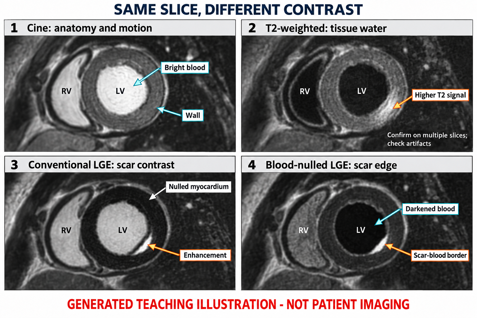
1 · Cine: bright blood outlines the myocardium; use a loop to assess contraction, not this still image.
2 · T2-weighted: a brighter myocardial region raises the question of edema; confirm location, source quality and complementary findings.
3 · Conventional LGE: the subendocardial bright band is a synthetic injury example; bright blood can make its inner edge difficult to see.
4 · Blood-nulled LGE: darker blood makes the scar–cavity border more conspicuous. The exact blood/myocardial appearance varies with technique.
Technical context:
Phase contrast measures velocity across a plane. Summing the vessel pixels gives flow rate, then integrating through the cardiac cycle gives volume. This original schematic includes reverse flow to explain the calculation. It is not a normal reference curve.
1 · Magnitude + phase: locate the vessel on magnitude images, track its contour each frame, and check phase direction, VENC, aliasing and offsets. Black versus white has no universal direction.
2 · Velocity to flow: sum velocity × pixel area across the lumen. Integrate flow rate over time to obtain volume.
3 · Use the right denominator: direct semilunar regurgitant fraction = reverse / forward × 100%. Indirect MR fraction = (LV stroke volume − aortic forward volume) / LV stroke volume × 100%.
4 · Reconcile: compare flow with ventricular volumes and the clinical question. An attractive curve does not validate the acquisition.
Technical context:
What to look at
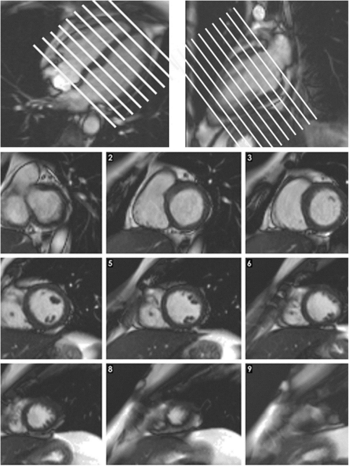
1. Top left and top right: Use both long-axis planes to prescribe the short-axis stack across the ventricles.
2. Bottom, slices 1–9: Scroll from base to apex and confirm complete LV and RV coverage.
3. Bottom, static frames: These are still frames from cine slices. Ventricular function and wall motion require the full cardiac cycle.
Published example, not a stand-alone diagnostic rule. Labels, scales and values belong to this acquisition.
What to look at
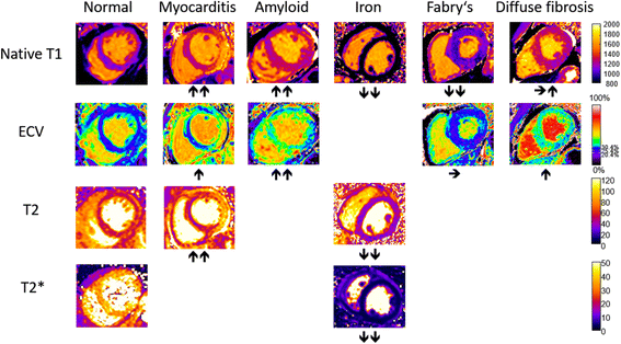
1. Native T1 row: T1 can rise with edema or amyloid and fall with iron or Fabry disease; interpret the pattern with the rest of the study.
2. ECV row: An expanded extracellular volume is a tissue signal, not a disease-specific diagnosis.
3. T2 and T2* rows: T2 increases with edema; iron shortens T2*. The sequences answer different questions.
4. Whole figure: Colors are display choices. Judge quantitative values against the scanner, sequence, field strength, and laboratory reference range.
Published example, not a stand-alone diagnostic rule. Labels, scales and values belong to this acquisition.
What to look at
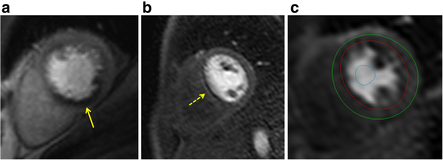
1. a: The inferior defect is subendocardial, more than one pixel wide, and follows a coronary territory.
2. b: The very thin, dark rim is an artifact example. The source notes onset before myocardial contrast arrival; confirm timing in the full series.
3. c: Red and green contours bound myocardium; the blue blood-pool ROI samples the input signal.
Published example, not a stand-alone diagnostic rule. Labels, scales and values belong to this acquisition.
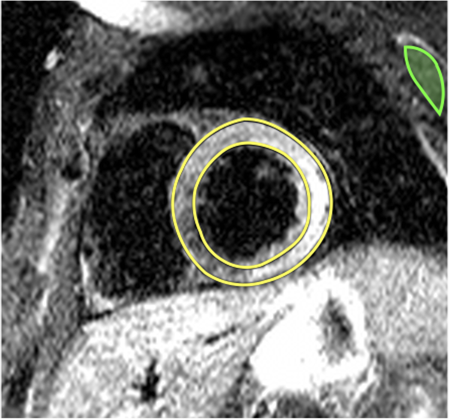
What to look at
1. Inferolateral and lateral wall: The brighter myocardial signal is the abnormal finding described in this acute myocarditis example.
2. Whole image: STIR is a qualitative T2-weighted image, not a quantitative T2 map in milliseconds.
3. Myocardial borders: Confirm that high signal is within myocardium and review for motion, coil, and slow-flow artifact before calling edema.
Published example, not a stand-alone diagnostic rule. Labels, scales and values belong to this acquisition.
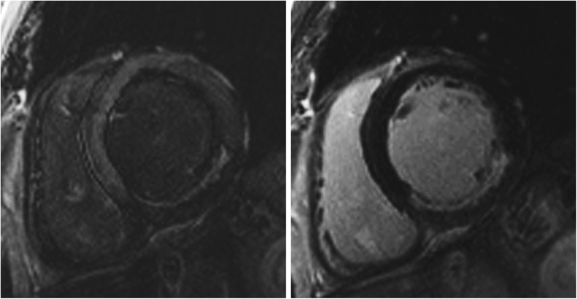
What to look at
1. Left: The etched appearance of normal myocardium signals a too-short inversion time; the inferior LGE is underestimated.
2. Right: Repeating with a longer inversion time reveals a larger inferior LGE zone.
3. Both panels: This is a technical acquisition comparison, not interval scar progression. These are magnitude images, not PSIR.
Published example, not a stand-alone diagnostic rule. Labels, scales and values belong to this acquisition.
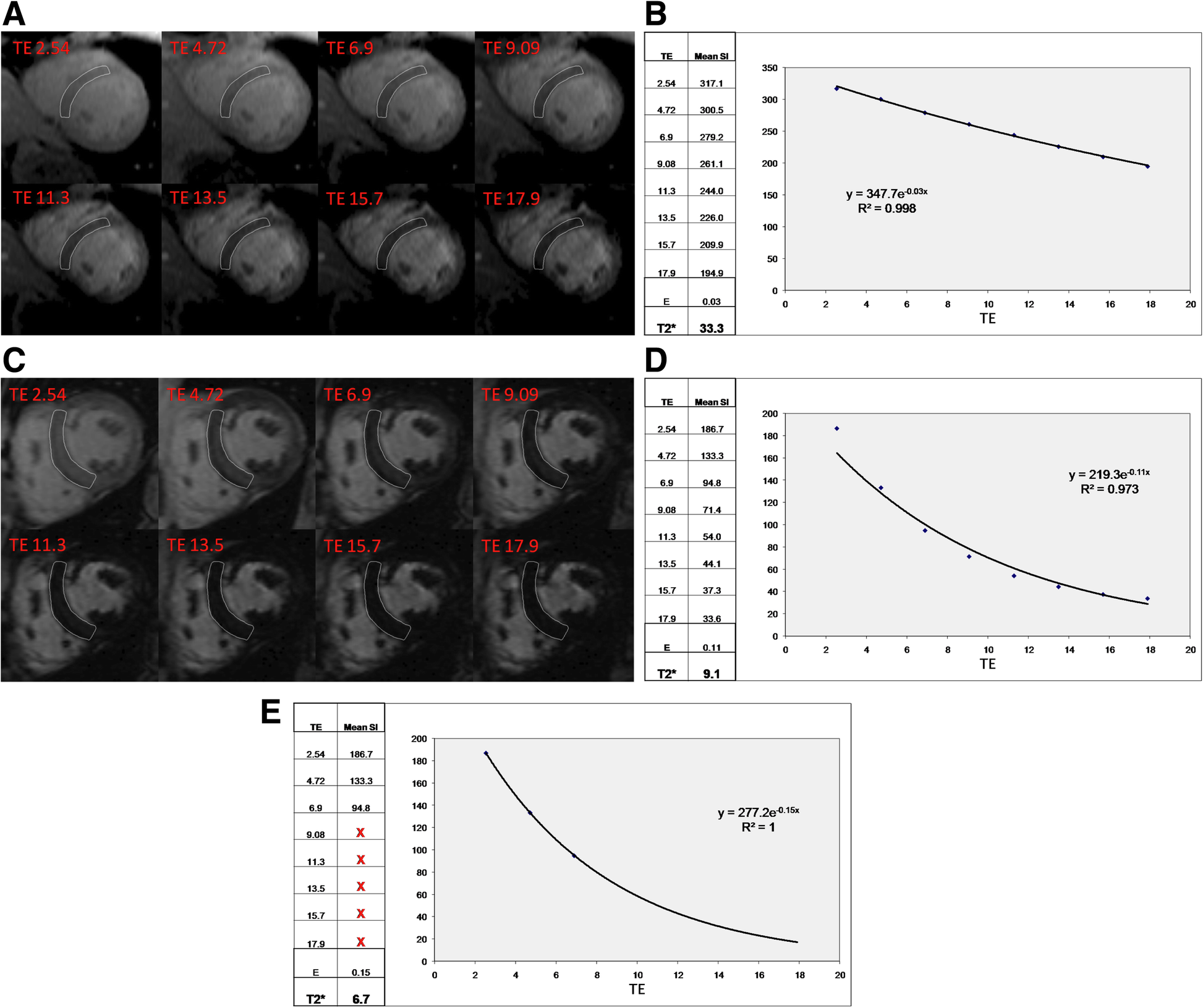
What to look at
1. a–b: Normal myocardium retains signal longer; the illustrated fitted T2* is 33.3 ms.
2. c: The iron-overloaded myocardium loses signal rapidly as TE increases.
3. d–e: Late echoes near the noise floor can bias the decay fit. Truncation changes the illustrated estimate from 9.1 to 6.7 ms.
4. Quantitative interpretation: Use a validated myocardial ROI and fitting method. Common <20 ms and <10 ms clinical thresholds apply to validated 1.5 T methods.
Published example, not a stand-alone diagnostic rule. Labels, scales and values belong to this acquisition.
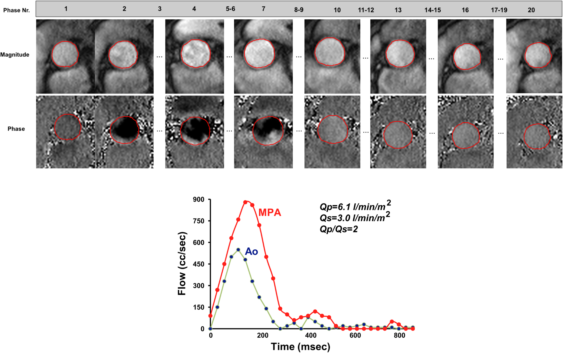
What to look at
1. Top, magnitude frames: Use anatomy to place and track the vessel contour through the cardiac cycle.
2. Top, phase frames: Phase carries velocity information. Bright/dark direction depends on the acquisition convention and must be checked.
3. Bottom: Integrating the flow curves gives pulmonary and systemic flow; Qp exceeds Qs in this illustrated VSD with left-to-right shunting.
Published example, not a stand-alone diagnostic rule. Labels, scales and values belong to this acquisition.
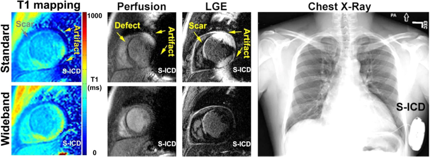
What to look at
1. Top versus bottom, T1 mapping: The conventional map is distorted near the device; wideband imaging reduces the artifact in the corresponding map.
2. Top versus bottom, perfusion and LGE: Device-related signal changes can resemble a perfusion defect or scar. Compare the corresponding wideband images.
3. Right: The chest radiograph shows the subcutaneous ICD responsible for the adjacent field disturbance.
Published example, not a stand-alone diagnostic rule. Labels, scales and values belong to this acquisition.
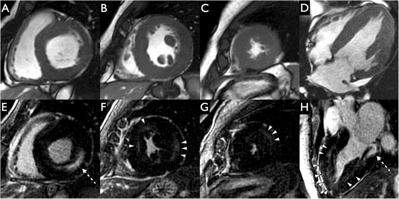
What to look at
1. A–D — Cine SSFP: First describe the concentric wall thickening and papillary muscles. These panels show morphology, not a dedicated scar acquisition.
2. E and H — Dashed arrows: Locate bright inferolateral midwall LGE. Its position within the wall is the key feature.
3. F–H — Arrowheads: Additional midwall enhancement shows that Fabry involvement need not be confined to one basal segment.
Published example, not a stand-alone diagnostic rule. Labels, scales and values belong to this acquisition.
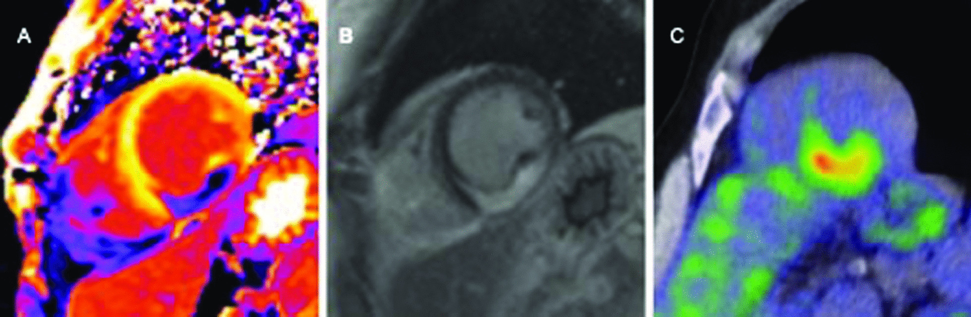
What to look at
1. A — Postcontrast T1 map: This is a postcontrast map, not native T1. Interpret only with its acquisition and contrast context.
2. B — Intramural bright signal: Identify the intense intramural LGE described by the authors; LGE characterizes myocardial injury.
3. C — Focal FDG uptake: PET adds metabolic information. Its interpretation requires appropriate myocardial suppression and clinical context.
Published example, not a stand-alone diagnostic rule. Labels, scales and values belong to this acquisition.
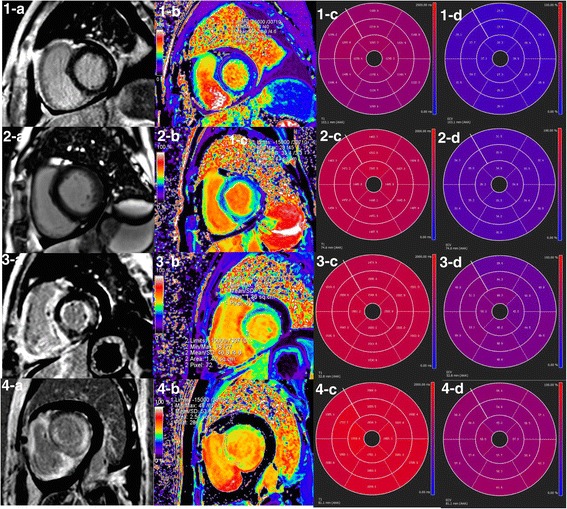
What to look at
1. 1-a versus 2-a — Both lack obvious LGE: The second row is an amyloidosis example despite no visible LGE; a negative LGE image does not exclude diffuse involvement.
2. 3-a and 4-a — Patchy versus global enhancement: Describe the LGE distribution before assigning an etiology.
3. Rows 2–4, columns c and d — Native T1 and ECV summaries: The authors report increased native T1 and ECV. Use local reference ranges; these printed values are not portable diagnostic thresholds.
Published example, not a stand-alone diagnostic rule. Labels, scales and values belong to this acquisition.
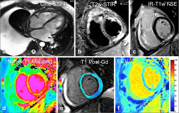
What to look at
1. a — Cine SSFP: Describe ventricular morphology and the pleural effusion. Functional interpretation uses the entire cine, not one frame.
2. b and c — T2-STIR and LGE: Look for corresponding inferior-wall subepicardial high signal. Edema and nonischemic injury are separate observations.
3. d–f — Native T1, postcontrast T1, and ECV: Compare like locations. ECV combines myocardial and blood T1 before/after contrast with hematocrit; a bright map alone is not a diagnosis.
Published example, not a stand-alone diagnostic rule. Labels, scales and values belong to this acquisition.
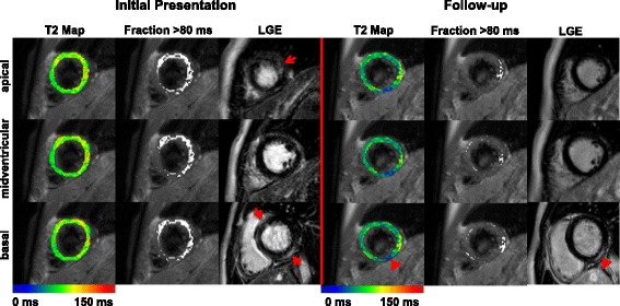
What to look at
1. Initial Presentation, LGE column — Red arrows: Locate the initial enhancement at the marked levels; then compare the same slice positions at follow-up.
2. Follow-up, basal row — Red arrowheads: Persistent basal LGE coexists with lower, blue-coded T2 in the corresponding region.
3. T2 Map and Fraction >80 ms columns — Different displays of one measurement: The >80-ms overlay was specific to this study and sequence; it is not a universal clinical threshold.
Published example, not a stand-alone diagnostic rule. Labels, scales and values belong to this acquisition.
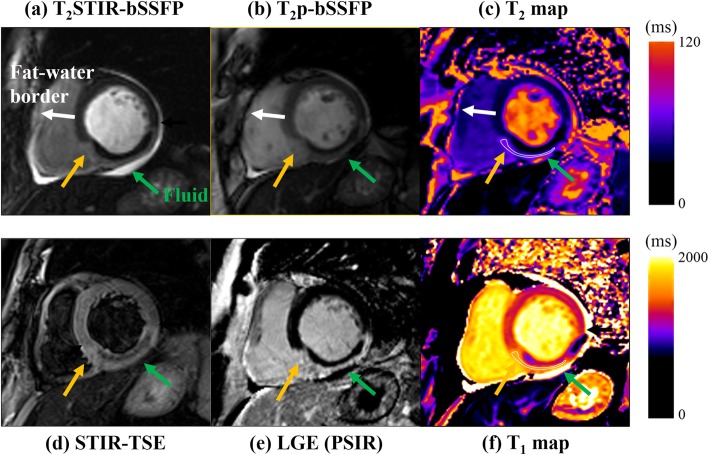
What to look at
1. c and f — T2 and T1 maps: Locate the abnormal region and compare the same myocardial location across the other sequences; both are measured in milliseconds, with different display ranges.
2. e — LGE: The dark core within the bright infarct was interpreted by the authors as most likely microvascular obstruction; compare its location with STIR (d).
3. a versus b — Fat suppression differs: The two bright-blood edema preparations do not make fat and fluid look identical. The sequence label is part of the interpretation.
Published example, not a stand-alone diagnostic rule. Labels, scales and values belong to this acquisition.
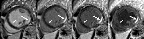
What to look at
1. Leftmost panel — Long arrow: Bright cavity blood competes with the subendocardial infarct signal, making the border less conspicuous.
2. Second through fourth panels — Long arrows: Increasing blood suppression separates the bright subendocardial lesion from the darker cavity.
3. Leftmost panel, short arrow — Septal blood-pool border: The source identifies Gibbs ringing that is not present on the dark-blood images; avoid calling this narrow border artifact scar.
Published example, not a stand-alone diagnostic rule. Labels, scales and values belong to this acquisition.
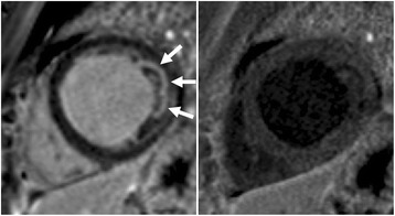
What to look at
1. Left panel — Three arrows: Inspect the apparently bright lateral subendocardial region; adjacent cavity/trabecular blood can mimic enhancement.
2. Right panel — Corresponding lateral border: With blood suppressed, the proposed lesion is no longer convincing. The authors identify the original signal as blood in trabeculae.
Published example, not a stand-alone diagnostic rule. Labels, scales and values belong to this acquisition.
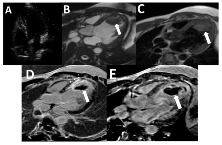
What to look at
1. B and C — Arrows: The apical mass is visible on cine and dark-blood images; morphology establishes its location.
2. D — Solid and dashed arrows: Standard LGE shows the thrombus and adjacent anteroseptal myocardial scar as separate findings.
3. E — Arrow; TI 600 ms in this study: The thrombus is homogeneously dark against enhancing tissue on the long-TI acquisition. The applicable TI depends on the protocol.
Published example, not a stand-alone diagnostic rule. Labels, scales and values belong to this acquisition.